Velocity Potential

We can elegantly define a velocity potential $\varphi (x,y,z)$ function that represents the velocity field as its gradient:

$$\mathbf{V}=\nabla \varphi$$

In component form:

$$\begin{array}{r}u=\frac{\partial \varphi }{\partial x}\\ v=\frac{\partial \varphi }{\partial y}\\ w=\frac{\partial \varphi }{\partial z}\end{array}$$

For a flow to be irrotational, the curl of the velocity vector must be zero:

$$\nabla \times \mathbf{V}=0$$

If $\mathbf{V}=\nabla \varphi$, then

$$\nabla \times (\nabla \varphi )=0$$

This is always true, because the curl of a gradient is always zero. This is why $\varphi$ is a valid representation of velocity for irrotational flows.

Laplace’s Equation for Potential Flows

For an incompressible flow:

$$\nabla \cdot \mathbf{V}=0$$

Substituting the velocity potential representation:

$$\nabla \cdot (\nabla \varphi )={\nabla }^2\varphi =0$$

This is Laplace’s Equation:

$$\frac{{\partial }^2\varphi }{\partial x^2}+\frac{{\partial }^2\varphi }{\partial y^2}+\frac{{\partial }^2\varphi }{\partial z^2}=0$$

Flows that satisfy this equation are known as potential flows. The beauty of this is that solving Laplace’s Equation, which is linear, gives us the entire velocity field.

Stream Function vs. Velocity Potential

How does the Stream Function compare to the Velocity Potential?

Stream function:

• Valid for 2D flows only
• Represents streamlines
• Consequence of mass conservation for incompressible flows
• Satisfies ${\nabla }^2\psi =0$

Velocity potential:

• Valid for 2D and 3D flows
• Represents equipotential lines (lines of constant velocity potential)
• Guaranteed by irrotationality
• Satisfies ${\nabla }^2\varphi =0$

A constant value of the stream function $\psi$ represents a streamline, describing the slope of the path traced by fluid particles

$$\psi =\text{const}⟹\frac{dy}{dx}=\frac{v}{u}$$

A constant value of $\varphi$ represents an equipotential line, describing lines of constant velocity potential

$$\varphi =\text{const}⟹udx+vdy=0$$

Lines of constant $\varphi$ (equipotentials) are always orthogonal to lines of constant $\psi$ (streamlines).

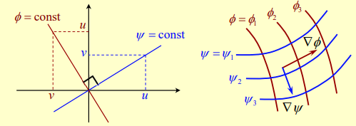
Mathematically, we can derive the orthogonality condition from the dot product of the gradients:

$$\nabla \varphi \cdot \nabla \psi =\frac{\partial \varphi }{\partial x}\frac{\partial \psi }{\partial x}+\frac{\partial \varphi }{\partial y}\frac{\partial \psi }{\partial y}=-uv+uv=0$$