Discretized Plant

Discretized Plant

To discrete a plant $C(s)$ with poles ${\lambda }_i$, we use

$$G[z]=\sum _{i=1}^n\frac{c_i}{{\lambda }_i}\frac{e^{{\lambda }_{i}T}-1}{z-e^{{\lambda }_{i}T}}$$

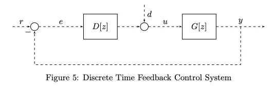
Consider a standard sampled-data feedback control system:

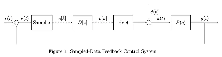
Here, we have $e(t)=r(t)-y(t)$ and a sampled $e[k]=e(kT)$.

We can consider another architecture:

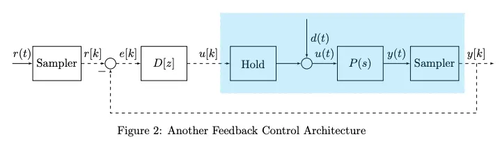
In this case, we have $y[k]=y(kT)$, $r[k]=r(kT)$, and $e[k]=r[k]-y[k]$.

It turns out that the two architectures above are actually equivalent. Then, let’s zoom into the blue part, which is a discretized plant.

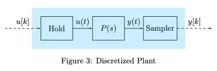
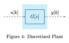
This discretized plant subsystem is DT LTI! Thus, we combine it into one $G[z]$:

Now, let’s think about a standard discrete time control system:

This system DT LTI. There is no approximation at the sample points. We know that sampled-data systems are not LTI, but this system is DT LTI. How is this possible? The discrete time control system is only valid (matches the DT system) only at the sample points. It determines behavior at the sample points only, not valid in between sample points

Thus, we aim to do direct design of $D[z]$ using the discretized plant $G[z]$. We will have:

• Transient specs guaranteed to be satisfied at the sample points
• Closed-loop stability guaranteed at sample points.

Thus, our goal is to derive $G[z]$ from $P(s)$, and show that is exact (an LTI system).

Assume that $P(s)$ has only simple poles and no integrator:

$$P(s)=\sum _{i=1}^n\frac{c_i}{s-p_i},p_i\ne 0\forall i$$

The sampler and hold do not have well-defined frequency domain representations since they are not LTI in general. Therefore, we must use time domain representations.

State space realization of $P(s)$:

$$\begin{array}{rl}\dot{x}& =\underset{A}{\underbrace{\left[\begin{array}{ccc}{p}_1& & \\ & \ddots & \\ & & p_n\end{array}\right]}}x+\underset{B}{\underbrace{\left[\begin{array}{c}1\\ ⋮\\ 1\end{array}\right]}}u\\ y& =\underset{C}{\underbrace{\left[\begin{array}{ccc}{c}_1& \dots & c_n\end{array}\right]}}x\end{array}$$

We can then write:

$$C(sI-A{)}^{-1}B=P(s)$$

This choice of state space is easy to solve since $A$ is diagonal so the states are decoupled. Between samples $u(t)$ is constant, such that:

$${\dot{x}}_i=p_i{x}_i+u_0\forall i$$

where $u_0$ is the constant value of $u(t)$ between samples.

Taking the Laplace transform with initial conditions:

$$\begin{array}{rl}s{X}_i(s)-(x_i{)}_0& =p_i{X}_i(s)+\frac{u_0}{s}\\ X_i(s)& =\frac{(x_i{)}_0}{s-p_i}+\frac{u_0}{s(s-p_i)}\\ & =\frac{(x_i{)}_0}{s-p_i}+\frac{u_0}{p_i}\left(\frac{1}{s-p_i}-\frac{1}{s}\right)\end{array}$$

where $x_0$ is the initial value of $x(t)$ just after the first sample.

Then, taking the inverse Laplace transform gives us:

$$\begin{array}{rl}{x}_i(t)& =e^{p_{i}t}(x_i{)}_0+\frac{u_0}{p_i}(e^{p_{i}t}-1)\forall i\\ x(t)& =\underset{e^{At}}{\underbrace{\left[\begin{array}{ccc}{e}^{p_{1}t}& & \\ & \ddots & \\ & & e^{p_{n}t}\end{array}\right]}}{x}_0+\underset{A^{-1}}{\underbrace{{\left[\begin{array}{ccc}{p}_1& & \\ & \ddots & \\ & & p_n\end{array}\right]}^{-1}}}\left(\underset{e^{At}}{\underbrace{\left[\begin{array}{ccc}{e}^{p_{1}t}& & \\ & \ddots & \\ & & e^{p_{n}t}\end{array}\right]}}-\underset{I}{\underbrace{\left[\begin{array}{ccc}1& & \\ & \ddots & \\ & & 1\end{array}\right]}}\right)\underset{B}{\underbrace{\left[\begin{array}{c}1\\ ⋮\\ 1\end{array}\right]}}{u}_0\\ x(t)& =e^{At}{x}_0+A^{-1}(e^{At}-I)B{u}_0\end{array}$$

Starting from $x_0=x[k]$ and $u_0=u[k]$ and find the solution after $t=T$ (one sampling period):

$$\begin{array}{rl}x[k+1]& =\underset{A_d}{\underbrace{e^{AT}}}x[k]+\underset{B_d}{\underbrace{A^{-1}(e^{AT}-I)B}}u[k]\\ x[k+1]& =A_{d}x[k]+B_{d}u[k]\end{array}$$

• Note: this system is DT LTI!

We want to find $G[z]$ in the frequency domain. Thus, using the $z$-transform:

$$\begin{array}{rl}zX[z]& =A_{d}X[z]+B_{d}U[z]\\ Y[z]& =CX[z]\end{array}$$

which gives:

$$\begin{array}{rl}X[z]& =(zI-A_d{)}^{-1}{B}_{d}U[z]\\ Y[z]& =CX[z]=C(zI-A_d{)}^{-1}{B}_{d}U[z]\end{array}$$

and

$$T_{uy}[z]=C(zI-A_d{)}^{-1}{B}_d=G[z]$$

which is the same result as for CT but with $s$ replaced by $z$. Thus,

$$\begin{array}{rl}G[z]& =C(zI-A_d{)}^{-1}{B}_d\\ & =\left[\begin{array}{ccc}{c}_1& \dots & c_n\end{array}\right]{\left[\begin{array}{ccc}z-e^{p_{1}T}& & \\ & \ddots & \\ & & z-e^{p_{n}T}\end{array}\right]}^{-1}\left[\begin{array}{ccc}\frac{1}{p_1}& & \\ & \ddots & \\ & & \frac{1}{p_n}\end{array}\right]\left[\begin{array}{ccc}{e}^{p_{1}T}-1& & \\ & \ddots & e^{p_{n}T}-1\end{array}\right]\left[\begin{array}{c}1\\ ⋮\\ 1\end{array}\right]\\ & =\left[\begin{array}{ccc}{c}_1& \dots & c_n\end{array}\right]\left[\begin{array}{ccc}\frac{1}{z-e^{p_{1}T}}& & \\ & \ddots & \\ & & \frac{1}{z-e^{p_{n}T}}\end{array}\right]\left[\begin{array}{c}\frac{1}{p_1}(e^{p_{1}T}-1)\\ ⋮\\ \frac{1}{p_n}(e^{p_{n}T}-1)\end{array}\right]\\ & =\left[\begin{array}{ccc}{c}_1& \dots & c_n\end{array}\right]\left[\begin{array}{c}\frac{1}{p_1}\frac{e^{p_1}T-1}{z-e^{p_{1}T}}\\ ⋮\\ \frac{1}{p_n}\frac{e^{p_n}T-1}{z-e^{p_{n}T}}\end{array}\right]\\ & =\sum _{i=1}^n\frac{c_i}{p_i}\frac{e^{p_{i}T-1}}{z-e^{p_{i}T}}\end{array}$$

where $G[z]$ is called the discretized plant.

• This is the same results as for c2d in MATLAB by coincidence, even though c2d is used for approximation whereas $G[z]$ is exact.

Note that the poles of $G[z]$ are at $\{e^{p_{1}T},\dots ,e^{p_{n}T}\}$, so they depend on both the poles of $P(s)$ and the sampling time $T$.

• As $T\to 0$, all poles approach $1$ (on the boundary of the unit disk). Thus, the system gets very slow and the control design becomes numerically unstable.
• However, $e^{p_{i}T}$ maps stable poles to stable poles – it preserves the stability type of each pole in $P(s)$ automatically.

Remember that $G[z]$ defines the behavior of the system at the sampling times. We need to look at Sampled-Data System Stability for behavior between sample times.