MA Kai Aimo (21195092)
1. Wheel Odometry
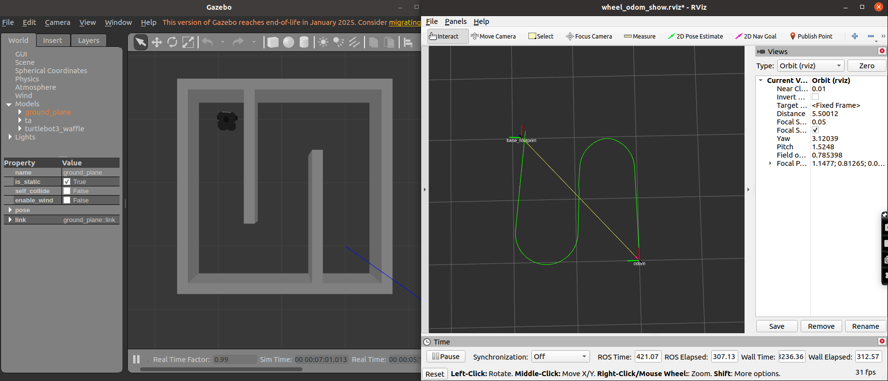
The node subscribes to joint state messages to obtain wheel rotations, computing the linear and angular displacement from the differences in wheel positions, and updating the robot’s global pose accordingly. The node then publishes both the updated path and odometry messages, including velocity estimates derived from time intervals between measurements.
Wheel odometry result:
2. Mapping
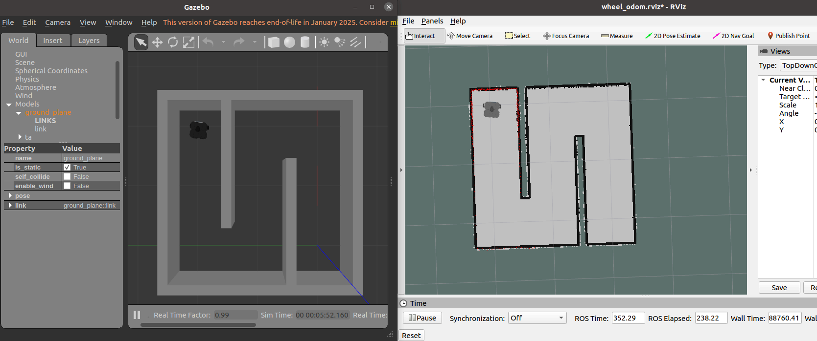
Laser scan measurements are transformed from the sensor’s frame into the map frame, aligning them with the robot’s base footprint and establishing a consistent spatial reference by initializing the map origin at the robot’s starting position. A Bresenham line algorithm [1] is used to trace the path of each laser beam, updating cell statuses by incrementing scan counts for endpoints and applying a decay mechanism for free space. Cells are marked as confirmed once their scan count surpasses a threshold. Finally, the occupancy grid is published.
Mapping result:
3. ICP Odometry
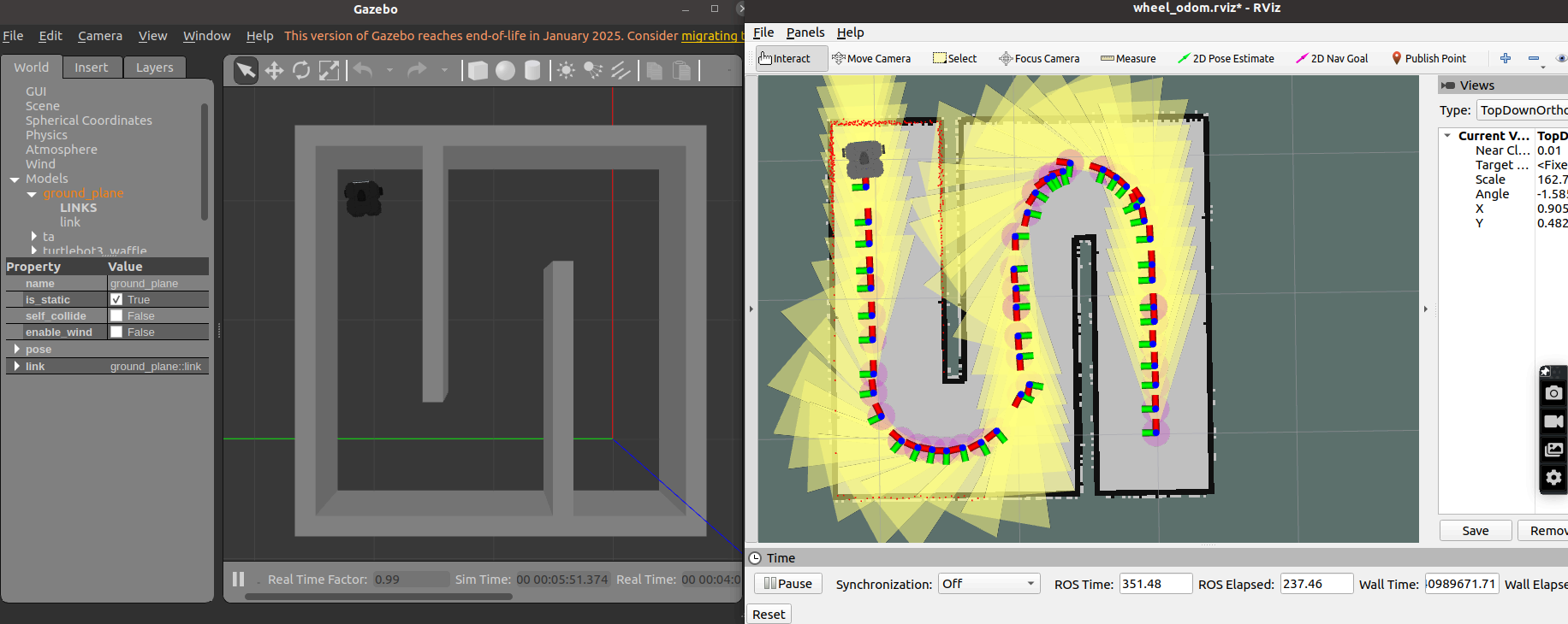
The occupancy grid map is turned into a point cloud by extracting cells that represent obstacles, and incoming laser scans are projected into the map frame. For each scan, the node transforms the laser data into a 2D point cloud using available tf transformations. Then, the ICP algorithm is applied to align the current scan’s point cloud with the obstacle map cloud. This process computes the optimal rigid transformation by matching corresponding points and minimizing the alignment error through centroid computation, cross-covariance analysis, and singular value decomposition (SVD). The updated transformation is broadcast as a new map-to-base transform, and an odometry message reflecting the refined pose is published.
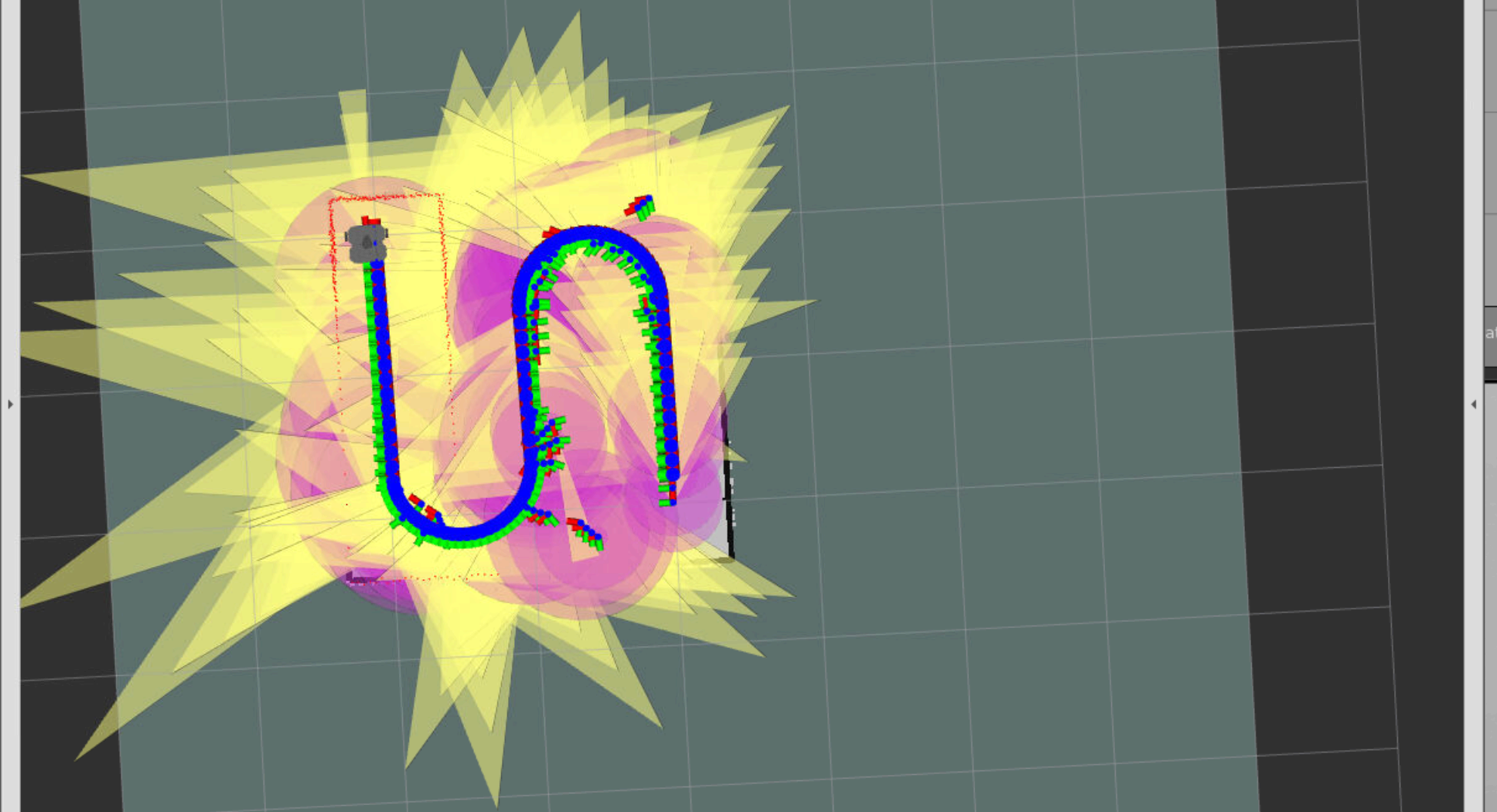
ICP odometry result:
4. Real-World
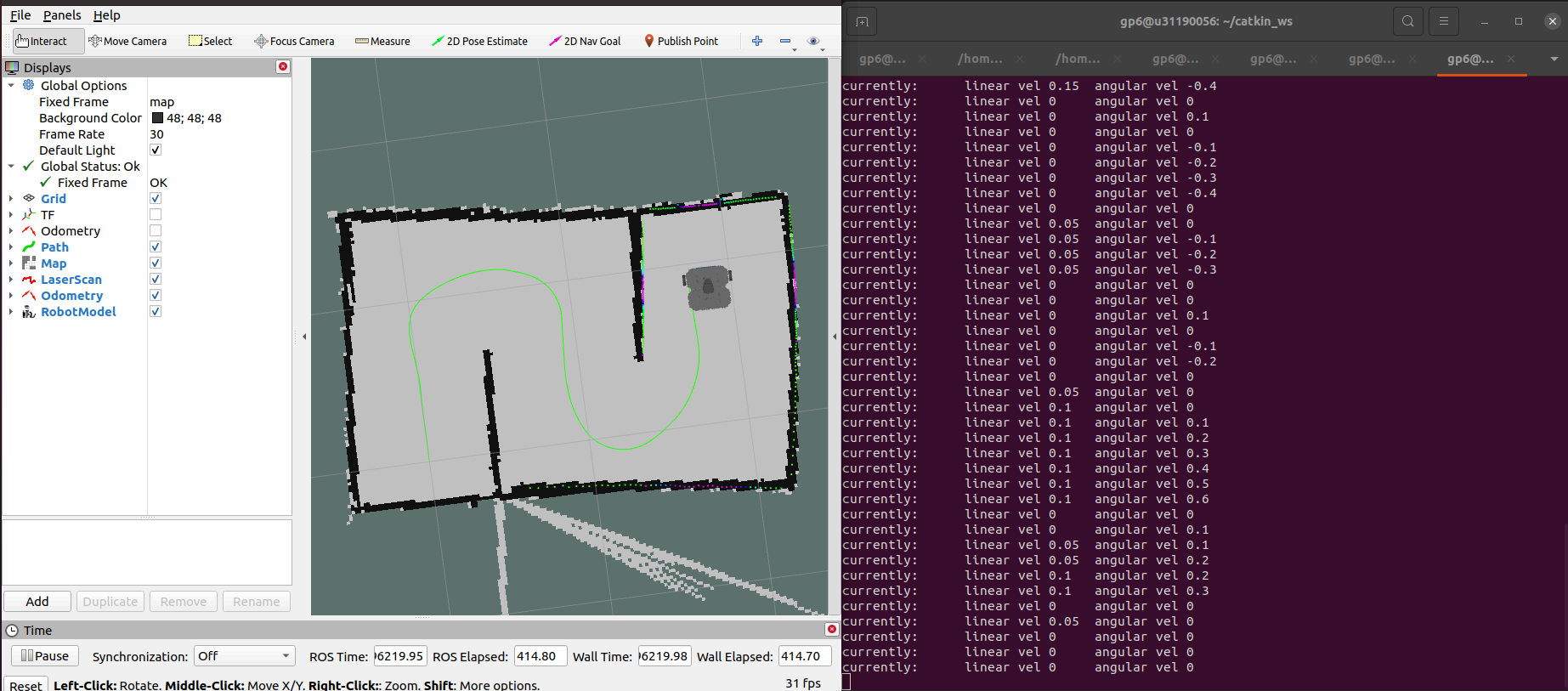
See video here: https://youtu.be/X82yDA6dX0Y. Path produced by wheel odometry is hard to see (visible at 00:30 - 00:40), and at 0:42 I accidentally input an extra space into the /robot_path topic name in RViz while trying to stop the robot, causing a RViz error.
Overall, the real-world performance of the above functionalities was comparable to the Gazebo simulation, with some discrepancies. First, the walls were not enclosed perfectly, leading to “streaks” appearing. The quality of wheel and ICP odometry was also generally slightly worse.
The wheel odometry path result is shown below, since it’s not readily visible in the video.
5. Bonus
5.1. Extended Kalman Filter
I implemented an Extended Kalman Filter [2] (see icpodom/ekf_odom.cpp) to use wheel odometry for motion prediction and refine it with ICP odometry corrections to improve localization accuracy. This takes advantage of high-frequency updates from wheel odometry and global corrections from ICP, while compensating for accumulating drift from wheel odometry, and slow speed from ICP. I found that this method functions much faster than just ICP, but still had occasional accuracy problems and inconsistent covariance.
5.2. Temporal Eigenvector Alignment
I also tried to create my own point-cloud registration method (see temporal_eigenvector_alignment.py). The main advantages of this method over ICP are that it does not require any correspondences or closest point matching, and it works on multiple point clouds whereas ICP only works on two point cloud at once.
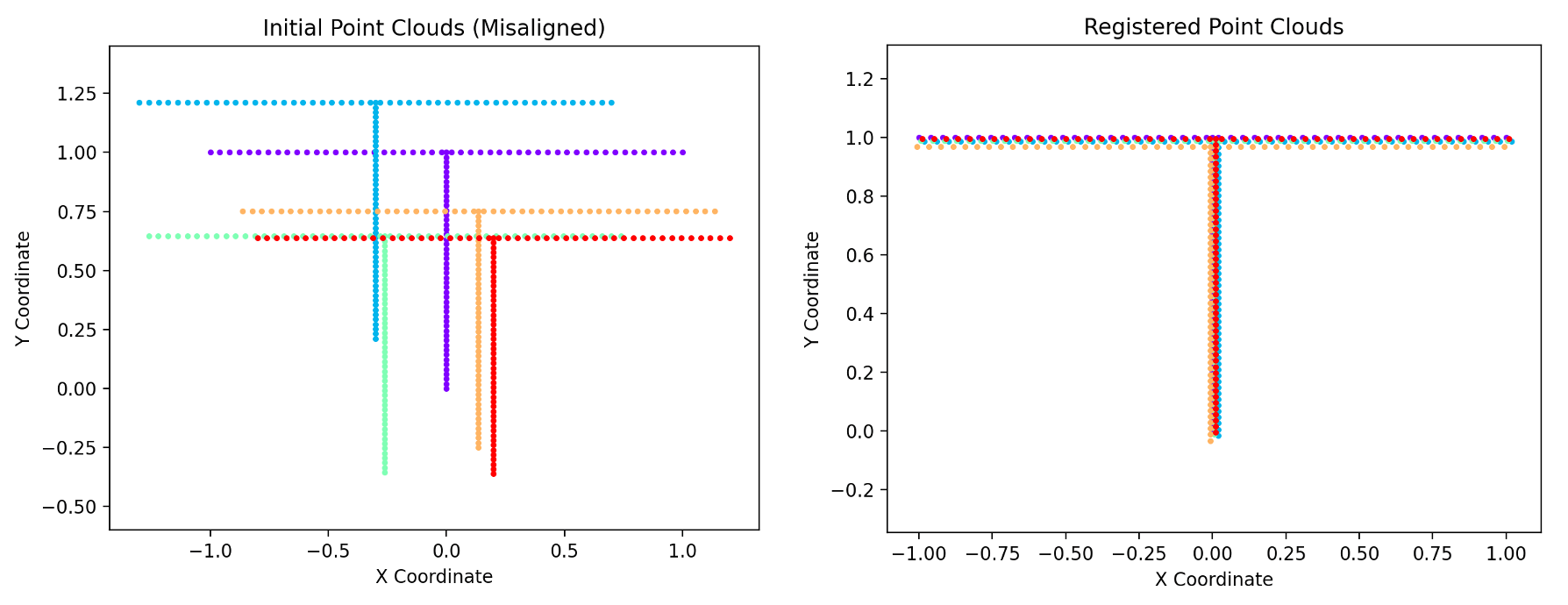
- Dataset: I created a toy dataset of ten T-shaped point clouds with random offsets, and the order of the points randomly shuffled (so no 1:1 correspondences). The point clouds are offset by simulating motion over time, and thus each point has and points move rigidly over time.
- Method: We treat the global covariance of all points (across all time steps) as our measure of ‘misalignment.’ By performing PCA on the aggregated point sets, we identify directions of largest spread. Stepping each point cloud’s transform in these directions reduces the overall spread, gradually converging to a minimal-variance alignment. This is an optimization-based approach similar to gradient descent; but instead of gradients, we descend along the eigenvectors to minimize variance. The core idea here is that the eigenvectors of a set of points basically denote the direction that variance occurs in those points, so stepping along the eigenvectors minimizes variance.
The below figure shows the point clouds before and after being aligned by my method; the registered point clouds align quite well. Point clouds are colorized by time.
I did some preliminary experiments with this method in the ROS simulation but the results were poor. It’s likely that being reliant on a global PCA may cause vulnerability to the noise or outliers in the point cloud, and the optimization could converge slowly or get stuck. More work would be needed to make this a reliable method for real applications.
References
[1] Bresenham, J. E. (1965). “Algorithm for computer control of a digital plotter”. IBM Systems Journal. 4 (1): 25–30. doi: 10.1147/sj.41.0025
[2] Pomerleau, François; Colas, Francis; Siegwart, Roland (2015). “A Review of Point Cloud Registration Algorithms for Mobile Robotics”. Foundations and Trends in Robotics. 4 (1): 1–104.
[3] Thrun, S., Burgard, W., & Fox, D. (2005). Probabilistic Robotics. MIT Press.