By definition, the analog signal is continuous and can take on any real value while digital signals are discrete and can only be integer values. Thus, converting between them requires some form of mapping, where a range of analog values are assigned to the same digital value (a binary code). As a result of this quantization, we have to deal with bias.
There are three ways of how we divide our signal if we are doing so linearly: round, take the floor, or take the ceiling of the input value. Each has bias involved.
The bias of the converter is not something selected by the user, rather it is inherent based on the selected converter design. For the hardware designs that will be considered in this course, none of them produce unbiased output. The outputs will always be biased high or biased low.
Rounding
A traditional rounding approach is shown below. Ideally, there would be a linear relationship as shown by the straight line. However, this is impossible and the actual relationship is a series of steps. In the unbiased case, if the analog value has a fractional portion when expressed in terms of LSB that is less than 0.5, round down (zones highlighted in red), otherwise round up (zones highlighted in blue).
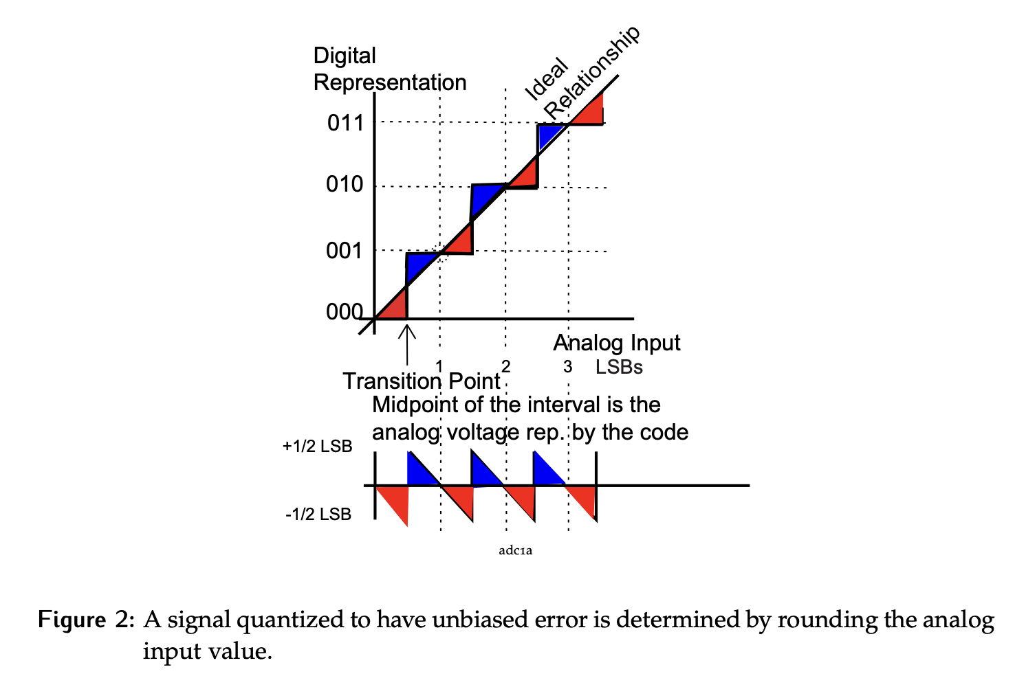
Consider the error with this approach:
- An input of 0.5 LSB would be rounded to 1, so the value is overestimated by 0.5 LSB.
- An input of 1 LSB would have no error.
- An input just shy of 1.5 will be underestimated the value by 0.5 LSB.
- As soon as the input crosses the 1.5 LSB line, the output is once again overestimating by 0.5 LSB.
Since the both overestimation and underestimation of the same magnitude are possible, it is referred to as unbiased error.
Floor
An alternative quantization scheme is to always take the floor of the analog value expressed in LSB.
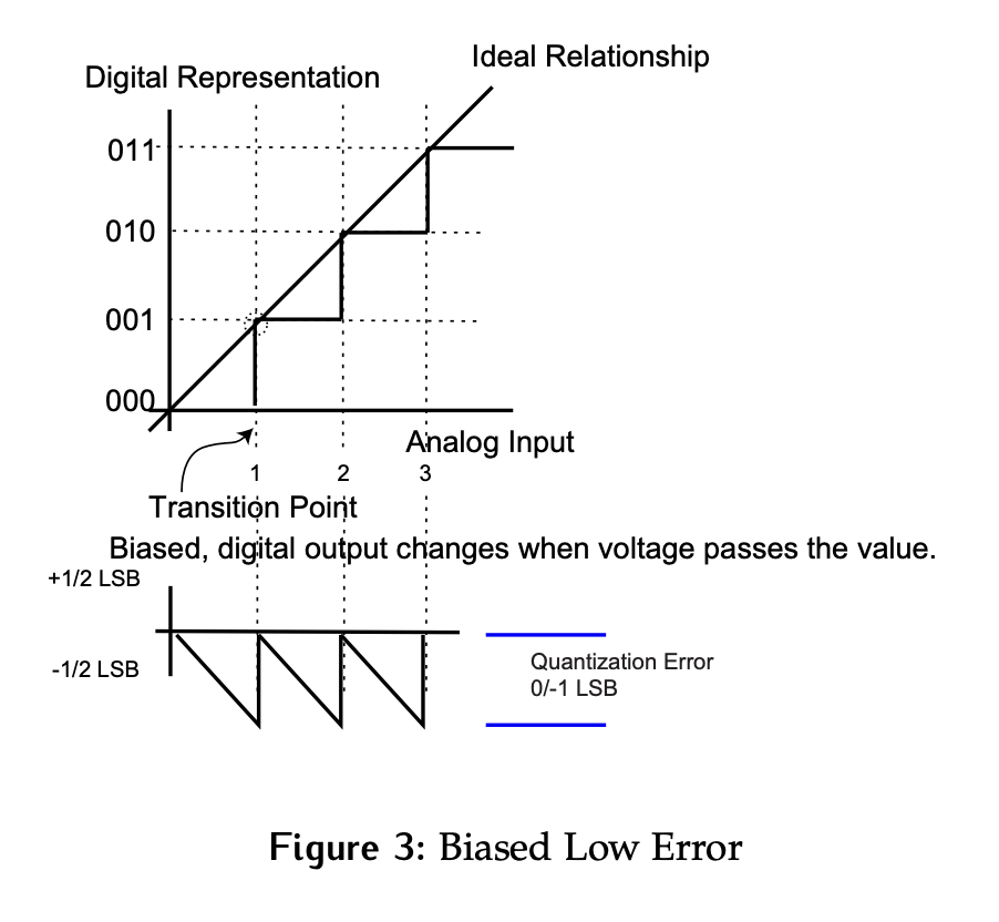
- In this case, any analog value between 0 and just shy of 1 LSB will be mapped to a digital value of 0, an analog value between 1 and just shy of 2 LSB will be mapped to a digital value of 1 etc.
- The error can once again be plotted, showing that there is no error at the edge of the step, say at 0 and that as the input increases towards the next transition point the error builds until it is just shy of 1 LSB and the output is underestimating by almost a whole LSB.
- Because this scheme always underestimates, it is referred to as biased low.
Ceiling
The opposite scheme would be to take the ceiling and always round up.
- If you were to plot the error in this case, the values would always be overestimated by 0 to just shy of 1 LSB.
- For this reason, this quantization scheme is referred to as biased high.