Phase 3 Tasks

Task 10: Programming Bandpass Filter Bank

We write a general function to generate a signal oscillating with the a certain frequency:

def generate_cosine_signal(freq, length, samplerate):
	t = np.arange(length) / samplerate
	return np.cos(2 * np.pi * freq * t)

Task 11: Amplitude Modulation

Similarly, a general function for amplitude modulation is written.

def amplitude_modulate(cosine_signal, rectified_signal):
	return cosine_signal * rectified_signal

Tasks 12 + 13: Output

Using the functions defined above, a cosine signal is generated for each band, oscillating around the central frequency of each band. Then, its amplitude is modulated using the rectified envelopes found in Phase 2. These signals are then all added together in order to generate an output signal; following the suggestion, this signal is normalized using the maximum of its maximum value. The sound is then played using the previously defined play_sound() function from Phase 1.

data, samplerate = get_audio_info('audio.mp3')
N = 20
bands = define_frequency_bands(N)
 
filtered_signals = [create_bandpass_filter(band, samplerate, filter_type='IIR')(data) for band in bands]
 
envelopes = [extract_envelope(signal, samplerate) for signal in filtered_signals]
 
modulated_signals = []
for i, band in enumerate(bands):
	central_freq = np.sqrt(band[0] * band[1]) # Calculate central frequency
	cosine_signal = generate_cosine_signal(central_freq, len(data), samplerate)
	modulated_signal = amplitude_modulate(cosine_signal, envelopes[i])
	modulated_signals.append(modulated_signal)
 
# Sum all signals for the output
output_signal = np.sum(modulated_signals, axis=0)
 
max_abs_value = np.max(np.abs(output_signal))
 
normalized_output_signal = output_signal / max_abs_value
 
play_sound(output_signal, samplerate)

Task 14: Initial Design Evaluation

Our design evaluation methodology (outlined in detail in phase 1) evaluates a given design by testing it across 8 audio samples. For each sample, a score between 0 and 5 is given by our team for the three categories of “Overall Clarity”, “Word intelligibility”, and “Similarity to original”. Thus, each filter has a maximum score of 120 (5 points * 3 categories * 8 audio samples = 120 points). To reduce bias, team members evaluated designs using a blind method, such that they are not aware of the design parameters of what they are grading.

Our initial design has the following parameters:

• N = 20 (20 frequency bands, split logarithmically, no overlap)
• Filter type: FIR
• Cut-off frequency: 400

This initial design performed poorly. While the general cadence of the audio could be heard, words were completely unintelligible and there was a lot of buzzing noise, leading to a low score of 27/120.

Task 15: Design Iterations

IIR vs FIR filters

The most significant factor found in our experimentation was the use of IIR vs. FIR filters. We originally used FIR filters for their linear phase response, which should theoretically lead to better stability and less distortion. However, we found that using FIR filters caused the output audio to be extremely garbled. This problem was only alleviated under two conditions:

• Very higher order (>500) FIR filters led to better outputs; however, they are much more computationally demanding and thus processing took much longer.
• Higher cutoff frequency for the envelope detection low-pass filter sometimes led to better outputs, but not consistently (only for certain audio samples). The improvement was also not very significant.

In general, we found that IIR filters were much more robust, with the added benefit of less computational requirements; using IIR for bandpass filtering had an especially large effect, with less difference in performance for the low-pass filter step of the envelope. Keeping our original design (N = 20 with logarithmic splits and no overlap, cut-off frequency = 400 Hz) but replacing the FIR filters with IIR filters led to a much higher score of 96/120, and much faster processing times.

Spacing Types

An initial experiment we conducted was to change the type of spacing. Our original design used logarithmic spacing as this aligns with the natural processing of the human cochlea; here, we experimented with linearly spaced bands by writing a define_linear_frequency_bands() function:

def define_linear_frequency_bands(N, min_freq=100, max_freq=8000):
	# Linearly space the band edges
	linear_band_edges = np.linspace(min_freq, max_freq, N+1)
	# Create bands based on these edges
	bands = [(linear_band_edges[i], linear_band_edges[i+1]) for i in range(N)]
	
	return bands

As expected, linear frequency bands have uniform coverage across the frequency spectrum. This led to better performance for musical audio, as it was easier to discern changes in pitch. However, there was a downgrade in performance for speech; this is likely due to the fact that speech elements like consonants are concentrated in higher frequency ranges. Thus, the scoring for this iteration (N = 20, split linearly, no overlap, cut-off frequency = 400 Hz, IIR filters) was slightly lower (89/120), as there are more speech samples (6) than music samples (2) in our testing set. We believe this is appropriate, as speech is more important to every day life than music for most users.

Overlapping sub-bands

We experimented with different overlaps of frequency bands. We found that adding small overlaps (10-30%) created a smoother and more natural sound, likely because this ensures a more continuous coverage of the frequency spectrum, reducing gaps. Qualitatively, we found that small overlaps led to better clarity of spoken words, especially in audio samples with background noise.

However, too much overlap between bands caused muddy sound quality and reduced the clarity of outputs. The cause of this is unclear, but it may be due to inter-channel interference of some kind.

• 10% overlap – score of 102/120.
• 30% overlap – score of 100/120.
• 70% overlap – score of 84/120.

Envelope LPF cut-off frequency

The low-pass filter in envelope detection extracts the amplitude envelope of the signal by filtering out high-frequency components and retaining the slowly varying amplitude changes that are crucial for speech perception. Thus, the cut-off frequency essentially determines the temporal resolution of the signal.

We found that setting the cut-off frequency too low (<400) lost important temporal details, leading to a muffled or unclear perception, especially for speech. This particularly affected the consonants and the overall naturalness of the sound. On the other hand, if the cut-off frequency is too high (>2000), the LPF allows of the fast-changing frequency components to pass through. This made the sound overly complex and harsh. We found the overall best cut-off frequency to be 700 Hz. This configuration (N = 20, logarithmic split, 10% overlap, IIR, 700 Hz cut-off) got a score of 106/120.

Task 16: Number of Channels

We found 20 channels to be an ideal number. Reducing the number of channels in worse resolution across the frequency spectrum, leading to worse understanding of speech, especially in audio samples with background noise. This also limited music perception. On the other hand, we found that increasing the number of channels past 20 had diminishing returns. While output quality did improve, this improvement was not significant, especially when considering that more channels leads to more processing requirements, which leads to more hardware requirements and worse battery life.

Some experiments:

• N = 5, logarithmic split, 10% overlap, IIR, 700 Hz cut-off – 62
• N = 10, logarithmic split, 10% overlap, IIR, 700 Hz cut-off – 84
• N = 15, logarithmic split, 10% overlap, IIR, 700 Hz cut-off – 93
• N = 20, logarithmic split, 10% overlap, IIR, 700 Hz cut-off – 106
• N = 25, logarithmic split, 10% overlap, IIR, 700 Hz cut-off – 109
• N = 40, logarithmic split, 10% overlap, IIR, 700 Hz cut-off – 105

As can be seen from the results, lower numbers of channels led to significantly worse performance, while higher numbers of channels did not lead to significant improvement.

Recommended Design

• N = 20 (number of channels)
  • Split logarithmically
  • 10% overlap between channels
• IIR filters for bandpass filter and envelope detection low-pass filter
• 700 Hz cut-off frequency for envelope detection low-pass filter
• Score: 106/120

Bonus: Quantitative Evaluation

We researched methods for quantitative evaluation based on statistical methods. Specifically, we wanted to find a way to compare the processed signal to the original signal. A good measure for this, found through our research, is the Pearson Correlation Coefficient, which measures the strength and direction of a linear relationship between two variables. It outputs a number between $-1$and $+1$, where a coefficient of $+1$ implies a perfect positive linear relationship, a coefficient of $0$ implies no relationship, and a coefficient of $-1$ implies a negative linear relationship. This was implemented using the scipy library:

from scipy.stats import pearsonr
 
def evaluate_output(original_signal, processed_signal):
	correlation, _ = pearsonr(original_signal, processed_signal)
	return correlation
 
correlation_coefficient = evaluate_output(data, normalized_output_signal)
print("Pearson Correlation Coefficient:", correlation_coefficient)

We found that our processed signals tend to have low correlations with the original signal, no matter the quality of the design. For example, our recommended filter design (qualitative score of 106/120) above only had a coefficient of $0.005864252262662308$. This indicates that these filters are universally poor at preserving audio information, which is consistent with our qualitative findings; even our best designs still sound significantly worse than original audio. Videos found online of cochlear implants output sound that was similar to ours, indicating that while cochlear implants are a great solution for people with difficulty hearing, they are still very far off from natural hearing.

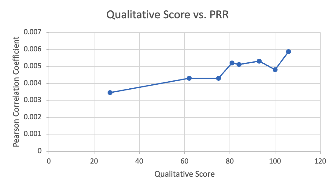
However, despite the universally low results, the Pearson Correlation Coefficient still quantifies the difference in quality between filter designs. For example, our original filter design, which had a low qualitative score of 27/120, had a PRR of $0.003447169795296812$. There seemed to be an approximately linear relationship between our qualitative scores and PRR, although there were plenty of outliers. This makes sense, as our qualitative scores are judged by team members and thus are prone to human error. It should be noted that similarity to original signal also does not always correspond to a better qualitative experience for the user; for example, a higher cut-off frequency results in better temporal resolution, resulting in higher PRR, but can be noisy for listening purposes.