Project 2– Finite Element Analysis

Problem #1: Stepped Shaft under Axial Loading

The stepped shaft is divided into 3 finite linear elements ($e_1,e_2,e_3$), where each element corresponds to a stepped section of the shaft. This then corresponds to four nodes, each of which have deformation of ${\delta }_1,{\delta }_2,{\delta }_3,{\delta }_4$. We model each element to have two equal and opposite forces acting on its ends/nodes, $F_1$ and $F_2$. $P$ represents the internal axial force, where $P=\sigma A$. The stress $\sigma$ can in turn be modeled as a function of the strain using Hooke’s Law, which states that $\sigma =Eϵ$. Here, $ϵ$ represents he strain of each element as defined as the ratio of its deformation due to applied force to its original length, such that $ϵ=({\delta }_1-{\delta }_2)/L$.

The expression $ϵ=({\delta }_1-{\delta }_2)/L$ can e substituted into $\sigma =Eϵ$ to get $\sigma =E({\delta }_1-{\delta }_2)/L$. This can in turn be substituted into $P=\sigma A$ to get $P=\frac{EA}{L}({\delta }_1-{\delta }_2)$. To maintain equilibrium, we must have $\sum F=F_1+P=0$, which gives $F_1=-P=-\frac{EA}{L}({\delta }_1-{\delta }_2)$. Since $F_2$ is equal and opposite to $F_1$, we have $F_2=\frac{EA}{L}({\delta }_1-{\delta }_2)$.

Thus, the local stiffness matrix $k_{\text{local}}$​ for an element of length $L$ and area $A$ and Young’s Modulus is given by:

$$\left[\begin{array}{c}{F}_1\\ F_2\end{array}\right]=\left[\begin{array}{cc}k& -k\\ -k& k\end{array}\right]\left[\begin{array}{c}{\delta }_1\\ {\delta }_2\end{array}\right],k=\frac{EA}{L}$$

This matrix shows the force response at each end of the element due to a unit displacement at each end, considering applied axial forces. The $2\times 2$ matrix composed of $k$ and $-k$ values is the local stiffness matrix.

Using the values of $E=200\text{ GPa}$, we can find the value of $k$ for each the local stiffness matrix of each element. $L$ differs for each element and is directly given. $A$ can be found by taking the given diameter and calculating $\pi {\left(\frac{d}{2}\right)}^2$. We can thus construct our element stiffness matrices:

$$\begin{array}{rl}\frac{E{A}_1}{L_1}& =\frac{69\times 10^9\text{ Pa}\cdot \pi {\left(\frac{0.03}{2}\text{ m}\right)}^2}{0.08\text{m}}=609665324.34,[k_{e_1}]=\left[\begin{array}{cc}609665324.34& -609665324.34\\ -609665324.34& 609665324.34\end{array}\right],\\ \frac{E{A}_2}{L_2}& =\frac{69\times 10^9\text{ Pa}\cdot \pi {\left(\frac{0.02}{2}\text{ m}\right)}^2}{0.16\text{m}}=135481183.19,[k_{e_2}]=\left[\begin{array}{cc}135481183.19& -135481183.19\\ -135481183.19& 135481183.19\end{array}\right],\\ \frac{E{A}_3}{L_3}& =\frac{69\times 10^9\text{ Pa}\cdot \pi {\left(\frac{0.01}{3}\text{ m}\right)}^2}{0.24\text{m}}=22580197.24[k_{e_3}]=\left[\begin{array}{cc}22580197.24& -22580197.24\\ -22580197.24& 22580197.24\end{array}\right]\end{array}$$

Our global stiffness matrix has dimensions $4\times 4$ since we have $4$ nodes. We also need to consider boundary conditions; specifically, the left end of $e_1$ is fixed so there is no displacement (${\delta }_1=0$). Thus, we can remove the first row and first columns of the matrix.

$$K_{\text{global}}=\left[\begin{array}{cccc}1& 0& 0& 0\\ 0& k_{e_1}+k_{e_2}& -k_{e_2}& 0\\ 0& -k_{e_2}& k_{e_2}+k_{e_3}& -k{e}_3\\ 0& 0& -k_{e_3}& -k_{e_3}\end{array}\right]$$

Thus, our full systems of equations is:

$$\begin{array}{rl}\{F\}& =[K]\{\delta \}\\ \left\{\begin{array}{c}0\\ 0\\ 0\\ 6100\end{array}\right\}& =\left[\begin{array}{cccc}1.00& 0.00& 0.00& 0.00\\ 0.00& 745146507.52& -135481183.19& 0.00\\ 0.00& -135481183.19& 158061380.38& -22580197.24\\ 0.00& 0.00& -22580197.24& 22580197.24\end{array}\right]\left\{\begin{array}{c}{\delta }_1\\ {\delta }_2\\ {\delta }_3\\ {\delta }_4\end{array}\right\}\end{array}$$

This is solved using MATLAB by simply doing d = K_global \ F;

Solving gives:

$$\left\{\begin{array}{c}{\delta }_1\\ {\delta }_2\\ {\delta }_3\\ {\delta }_4\end{array}\right\}=\left[\begin{array}{c}0\\ 0.01001\\ 0.05503\\ 0.32518\end{array}\right]\times 10^{-3}$$

The stress and strain are then calculated based on the formulas introduced earlier:

$$\begin{array}{rl}\text{Strain:}& {ϵ}_i=\frac{{\delta }_{i+1}-{\delta }_i}{L_i}\\ \text{Stress:}& {\sigma }_i=E{ϵ}_i\end{array}$$

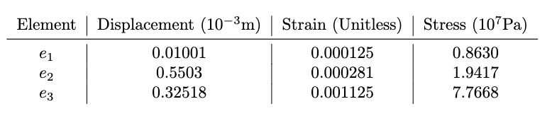
\The results are summarized in the table below.

To verify our FEA result, we can calculate deformations by hand using the deformation formula. They are given here:

$$\begin{array}{rl}{\delta }_1& =\frac{F{L}_1}{A_{1}E}=\frac{6100\text{ N}(0.08\text{ m})}{\pi {\left(\frac{0.03}{2}\text{ m}\right)}^2(69\times 10^9\text{ Pa})}=0.01001\times 10^{-3}\text{ m}\\ {\delta }_2& =\frac{F{L}_2}{A_{2}E}+{\delta }_1=\frac{6100\text{ N}(0.16\text{ m})}{\pi {\left(\frac{0.02}{2}\text{ m}\right)}^2(69\times 10^9\text{ Pa})}+0.01001\times 10^{-3}=0.05503\times 10^{-3}\text{m}\\ {\delta }_3& =\frac{F{L}_2}{A_{2}E}+{\delta }_2=\frac{6100\text{ N}(0.24\text{ m})}{\pi {\left(\frac{0.01}{2}\text{ m}\right)}^2(69\times 10^9\text{ Pa})}+0.05503\times 10^{-3}\text{ m}=0.32503\times 10^{-3}\text{m}\end{array}$$

These are consistent with our FEA calculations!

Problem #2: Deformation of a Truss Structure

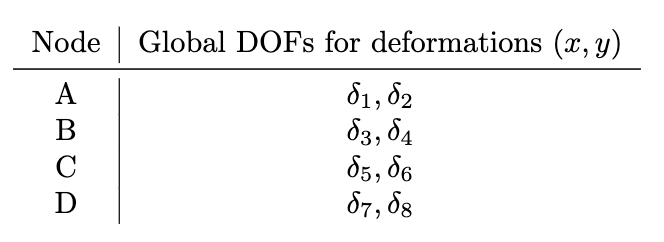
The truss comprises of four nodes. Each node ($A,B,C,D$) is defined by its coordinates in 2D space, with

$$A=(0,2),B=(4,2),C=(2,0),D=(0,0)$$

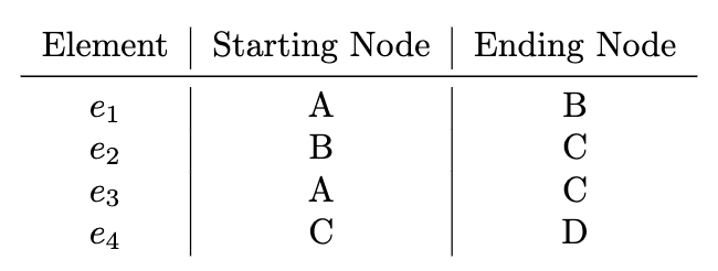
To build our FEA model, the elements of the truss are defined such that each member is an element (total of four elements). A connectivity matrix is then created to define how nodes are connected by elements. Each column in this matrix represents an element, and the two rows provide the start and end nodes for each element. For example, element 1 connects node A to node B, element 2 connects node B to node C, and so forth. To summarize, each element is defined as:

We also define the global degrees of freedoms; each node has 2 degrees of freedom ($x,y$). We use the notation of $\delta$ to indicate that these degrees of freedoms correspond to the deformations at each joint.

The length of each member is found:

$$\begin{array}{rl}{L}_1& =\sqrt{x^2+y^2}=\sqrt{4^2+0^2}=4\text{ m}\\ L_2& =\sqrt{x^2+y^2}=\sqrt{2^2+2^2}=2\sqrt{2}\text{ m}\\ L_3& =\sqrt{x^2+y^2}=\sqrt{2^2+2^2}=2\sqrt{2}\text{ m}\\ L_4& =\sqrt{x^2+y^2}=\sqrt{2^2+0^2}=2\text{ m}\end{array}$$

The local stiffness matrix for this problem how much a truss member/element resists deformation under applied forces. It links the forces at the nodes of an element to the displacements at those nodes. For 2D members, this matrix is defined as:

$$k_{\text{local}}=k_{e_i}\times \left[\begin{array}{cccc}\cos (\theta {)}^2& \cos (\theta )\sin (\theta )& -\cos (\theta {)}^2& -\cos (\theta )\sin (\theta )\\ \cos (\theta )\sin (\theta )& \sin (\theta {)}^2& -\cos (\theta )\sin (\theta )& -\sin (\theta {)}^2\\ -\cos (\theta {)}^2& -\cos (\theta )\sin (\theta )& \cos (\theta {)}^2& \cos (\theta )\sin (\theta )\\ -\cos (\theta )\sin (\theta )& -\sin (\theta {)}^2& \cos (\theta )\sin (\theta )& \sin (\theta {)}^2\end{array}\right]$$

where $k_{e_i}=EA/L$. This reflects the element’s response to axial, shear, and bending forces, assuming linear elastic behavior. By incorporating the directional cosines and cosines, the matrix is also in the global coordinate system without us needing to take an extra step to transform elements 2 and 3 to global coordinates. For our elements, we have:

$$\begin{array}{rl}{k}_{e_1}& =\frac{(200\times 10^9\text{ Pa})(400\times 10^{-6}\text{ m})}{4\text{ m}}=20000000,{\theta }_1=0\to [k_{e_1}]=\left[\begin{array}{cccc}20000000& 0& -20000000& 0\\ 0& 0& 0& 0\\ -20000000& 0& 20000000& 0\\ 0& 0& 0& 0\end{array}\right]\\ k_{e_2}& =\frac{(200\times 10^9\text{ Pa})(400\times 10^{-6}\text{ m})}{2\sqrt{2}\text{ m}}=14142135.62,{\theta }_2=135\to [k_{e_2}]=\left[\begin{array}{cccc}1.4142& 1.4142& -1.4142& -1.4142\\ 1.4142& 1.4142& -1.4142& -1.4142\\ -1.4142& -1.4142& 1.4142& 1.4142\\ -1.4142& -1.4142& 1.4142& 1.4142\end{array}\right]\times 10^7\\ k_{e_3}& =\frac{(200\times 10^9\text{ Pa})(400\times 10^{-6}\text{ m})}{2\sqrt{2}\text{ m}}=14142135.62,{\theta }_3=-135\to [k_{e_2}]=\left[\begin{array}{cccc}1.4142& -1.4142& -1.4142& 1.4142\\ -1.4142& 1.4142& 1.4142& -1.4142\\ -1.4142& 1.4142& 1.4142& -1.4142\\ 1.4142& -1.4142& -1.4142& 1.4142\end{array}\right]\times 10^7\\ k_{e_4}& =\frac{(200\times 10^9\text{ Pa})(400\times 10^{-6}\text{ m})}{2\text{ m}}=40000000,{\theta }_4=0\to [k_{e_4}]=\left[\begin{array}{ccccc}40000000& 0& -40000000& 0& \\ 0& 0& 0& 0& \\ -40000000& 0& 40000000& 0& \\ 0& 0& 0& 0& \end{array}\right]\end{array}$$

With these, the full local stiffness matrices can be found; they are omitted here for brevity. We can then integrate each element’s stiffness matrix into the global stiffness matrix, $K_{\text{global}}$. Since there are four nodes, and each node has 2 degrees of freedom, our global stiffness matrix has dimensions of $8\times 8$. The placement of each element’s stiffness matrix within $K_{\text{global}}$​ depends on the nodes that the element connects. This is guided by the connectivity matrix. For example, the connectivity matrix states that element 1 connects nodes A and B; thus, its local stiffness matrix affects the DOFs corresponding to these nodes in $K_{\text{global}}$​. Following this approach, the corresponding entries in $K_{\text{global}}$ are updated for each element by adding the element’s stiffness contributions to the appropriate positions in the global matrix. Finally, boundary conditions are applied to nodes A and D, which are fixed. Fixed nodes have their corresponding rows and columns in the global stiffness matrix set to zero, except diagonals are set to $1$.

$$K_{\text{global}}=\left[\begin{array}{cccccccc}1& 0& 0& 0& 0& 0& 0& 0\\ 0& 1& 0& 0& 0& 0& 0& 0\\ 0& 0& 3.4142& 1.4142& -1.4142& -1.4142& 0& 0\\ 0& 0& 1.4142& 1.4147& -1.4142& -1.4142& 0& 0\\ 0& 0& -1.4142& -1.4142& 6.8284& 0& 0& 0\\ 0& 0& -1.4142& -1.4142& 0& 2.8284& 0& 0\\ 0& 0& 0& 0& 0& 0& 1& 0\\ 0& 0& 0& 0& 0& 0& 0& 1\end{array}\right]\times 10^7$$

Due to the boundary conditions applied to node A (row/columns 1 and 2) and node D (row/columns 7 and 8), our original $8\times 8$ matrix can be simplified to $4\times 4$ so that our system of equations is:

$$\begin{array}{rl}\{F\}& =[K]\{\delta \}\\ \left\{\begin{array}{c}0\\ -51000\\ 0\\ 0\end{array}\right\}& =10^7\times \left[\begin{array}{cccc}3.4142& 1.4142& -1.4142& -1.4142\\ 1.4142& 1.4147& -1.4142& -1.4142\\ -1.4142& -1.4142& 6.8284& 0\\ -1.4142& -1.4142& 0& 2.8284\end{array}\right]\left\{\begin{array}{c}{\delta }_3\\ {\delta }_4\\ {\delta }_5\\ {\delta }_6\end{array}\right\}\end{array}$$

This is once again solved with MATLAB by setting up the matrices and calling d = K_global \ F;.

Then, the strains can be calculated for each member by considering its deformations at each of its nodes. Since each element has 2 nodes, which in turn each have 2 degrees of freedom for deformation, we have:

$$\text{Strains: }{ϵ}_i=\frac{-{\delta }_{{\text{start}}_x}\cdot \cos \theta -{\delta }_{{\text{start}}_y}\cdot \sin \theta +{\delta }_{{\text{end}}_x}\cos \theta +{\delta }_{{\text{end}}_y}\sin \theta }{L}$$

The stresses, internal forces, change in length, and factor of safety can then be calculated using:

$$\begin{array}{rl}\text{Stress: }& {\sigma }_i=E{ϵ}_i\\ & \\ \text{Internal forces: }& P_i=A_i\cdot {\sigma }_i\\ & \\ \text{Change in length: }& \Delta L_i=\underset{\text{Deformed length}}{\underbrace{\sqrt{(x_{\text{start}}+{\delta }_{{\text{start}}_x}-(x_{\text{end}}+{\delta }_{{\text{end}}_x}){)}^2+(y_{\text{start}}+{\delta }_{{\text{start}}_y}-(y_{\text{end}}+{\delta }_{{\text{end}}_y}){)}^2}}}-L\\ & \\ \text{Factor of safety: }& \text{F.S}=\frac{{\sigma }_{\text{yield}}}{|\sigma |}\end{array}$$

Results for these quantities are displayed below.

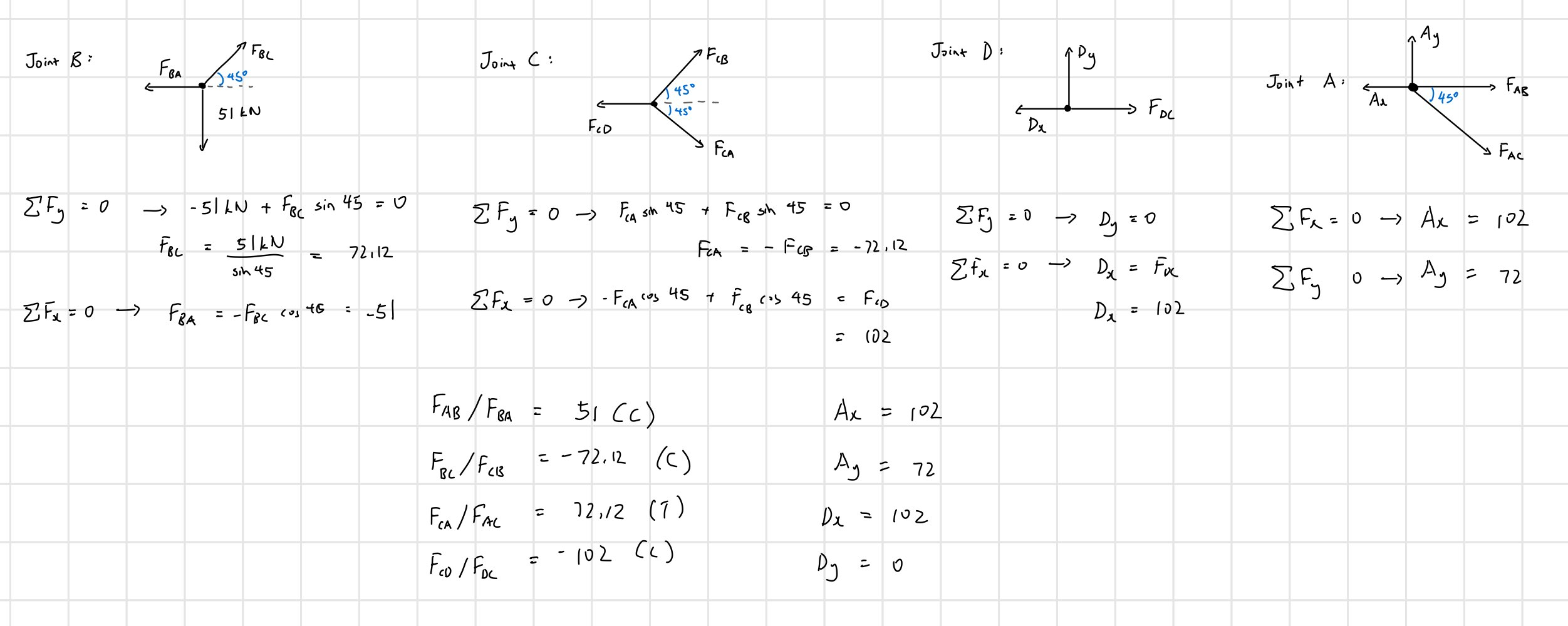
We can verify these by using the method of joints on the truss structure to calculate internal forces. The figure below shows this process.

Factor of Safety Recommendations

Given the factor of safety values of $1.9608,1.3865,1.3865,0.9804$ for the four truss elements, we see that Element 4 is unsafe. A factor of safety below $1$ indicates that the stresses in this member exceed its yield strength, suggesting a risk of failure under the given loading conditions. While the other members are relatively more safe with factors of safety above $1$, these can also be inadequate depending on the application, as some use cases typically require higher factors of safety (2 to 3). Some ways to increase factor of safety for individual members would be to increase the cross-sectional areas of the element, or simply use a material with a higher yield strength. A more drastic option would be to redesign the truss configuration entirely to redistribute loads more evenly.