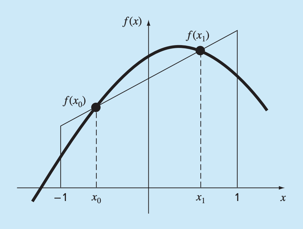
Gauss Quadrature

Gauss Quadrature (also known as Gauss-Legendre) employs values positioned between the evaluation/measured points to achieve an improved estimate of the integral. If we can ‘balance’ the positive and negative errors between the straight line approximation and the curve, we can achieve a better estimate of the integral.

Provides exact values of integrals for polynomials up to degree $2n-1$ (for n points). For example, 2 data points would be accurate for a polynomial up to degree $3$.

Two-Point Gauss-Legendre Formula

Using the method of undetermined coefficients - the area (integral) can be approximated as:

$$I\approx c_{0}f(x_0)+c_1(f(x_1))$$

where $c_0$ and $c_1$ are unknown coefficients, and $x_0$ and $x_1$ are fixed at the endpoints (4 unknowns requires 4 locations).

To develop 4 equations, we assume the 4 unknowns fit the
integrals of:

1. Constant function ($y=\text{constant}$)
2. Linear function ($y=x$)
3. Parabolic function ($y=x^2$)
4. Cubic function ($y=x^3$)

Let’s go through these step by step.

Constant function:

$$\begin{array}{r}{c}_{0}f(x_0)+c_{1}f(x_1)={\int }_{-1}^{1}1dx=2\\ c_0+c_1=2\end{array}$$

Linear function:

$$\begin{array}{r}{c}_{0}f(x_0)+c_{1}f(x_1)={\int }_{-1}^{1}xdx=0\\ \therefore c_0{x}_0+c_1{x}_1=0\end{array}$$

Parabolic function:

$$\begin{array}{r}{c}_{0}f(x_0)+c_{1}f(x_1)={\int }_{-1}^1{x}^{2}dx=\frac{2}{3}\\ \therefore c_0{x}_0^2+c_1{x}_1^2=\frac{2}{3}\end{array}$$

Cubic function:

$$\begin{array}{r}{c}_{0}f(x_0)+c_{1}f(x_1)={\int }_{-1}^1{x}^{3}dx=0\\ \therefore c_0{x}_0^3+c_1{x}_1^3=0\end{array}$$

These can be solved as:

$$\begin{array}{rl}{c}_0& =c_1=1\\ x_0& =-\frac{1}{\sqrt{3}}=-0.5773504\\ x_1& =\frac{1}{\sqrt{3}}=0.5773504\end{array}$$

This yields:

$$I\approx f\left(-\frac{1}{\sqrt{3}}\right)+f\left(\frac{1}{\sqrt{3}}\right)$$

A simple change of variable can be used to translate other limits of integration into this form. This is accomplished by assuming that a new variable $x_d$ is related to the original variable $x$ in a linear fashion, as in

$$x=a_0+a_1{x}_d$$

The lower limit $x=a$ corresponds to $x_d=-1$, such that we have:

$$a=a_0+a_1(-1)$$

Similarly, the upper limit $x=b$, corresponds to $x_d=1$, such that:

$$b=a_0+a_1(1)$$

These can then be solved with:

$$\begin{array}{r}{a}_0=\frac{b+a}{2},a_1=\frac{b-a}{2}\end{array}$$

which results in:

$$x=\frac{(b+a)+(b-a)x_d}{2}$$

which can in turn be differentiated to find:

$$dx=\frac{b-a}{2}d{x}_d$$

Two-point Example

Integrate $f(x)=x^4$ over the interval $0\le x\le 2$ with two-point Gauss Quadrature.

We have:

$$\begin{array}{r}I={\int }_0^2{x}^{4}dx={\int }_{-1}^1(1+x_d{)}^{4}d{x}_d\end{array}$$

where:

$$\begin{array}{r}x=\frac{b+a}{2}+\frac{b-a}{2}{x}_d=\frac{2+0}{2}+\frac{2-0}{2}{x}_d=1+x_d\end{array}$$

and

$$\begin{array}{rl}dx& =\frac{b-a}{2}d{x}_d=\frac{2-0}{2}d{x}_d=d{x}_d\end{array}$$

Thus:

$$I=f\left(x_d=-\frac{1}{\sqrt{3}}\right)+f\left(x_d=\frac{1}{\sqrt{3}}\right)$$

Solving:

$$\begin{array}{rl}f\left(x_d=\frac{1}{\sqrt{3}}\right)& ={\left(1+\frac{1}{\sqrt{3}}\right)}^4=6.19\\ f\left(x_d=-\frac{1}{\sqrt{3}}\right)& ={\left(1-\frac{1}{\sqrt{3}}\right)}^4=3.19\times 10^{-2}\\ I& =6.19+0.00319=6.22\end{array}$$

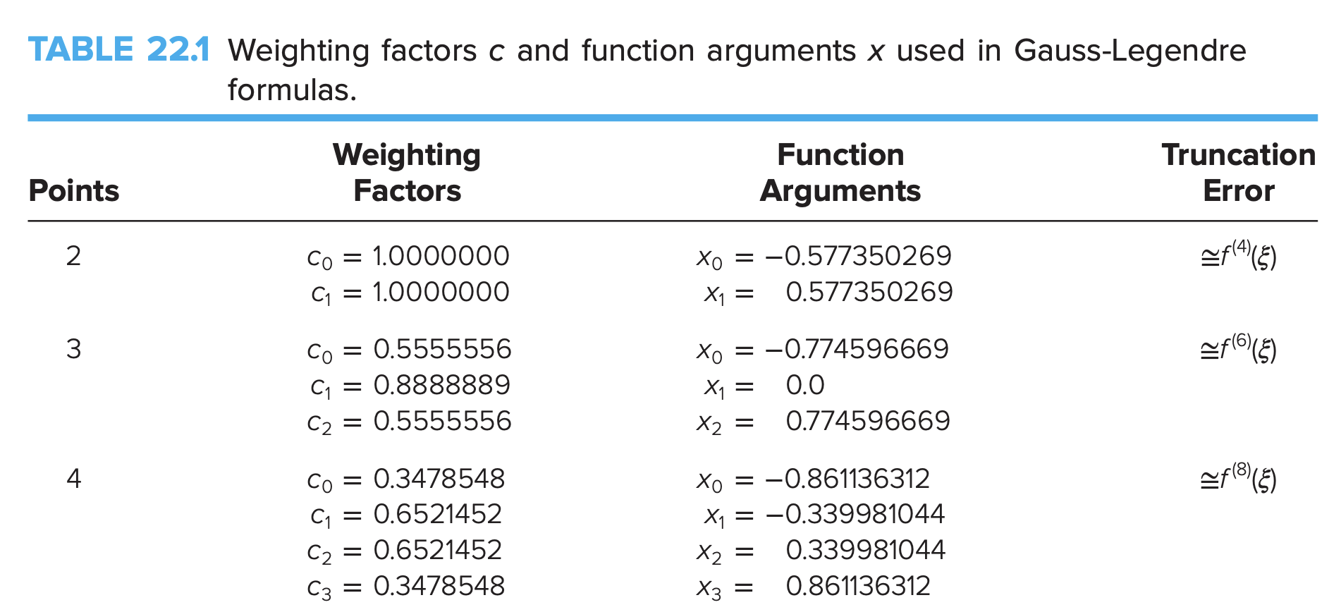
Higher-Order Gauss-Legendre

The general formulation is just:

$$I\approx c_{0}f(x_0)+c_1(f{x}_1)+\cdots +c_{n-1}f(x_{n-1})$$

Three-point Example

Integrate $f(x)=x^4$ over the interval $0\le x\le 2$ with 3-point Gauss Quadrature.

$$\begin{array}{r}{\int }_0^2{x}^{4}dx={\int }_0^2(1+x^4)d{x}_d\end{array}$$

Thus, we have:

$$I\approx 0.555556\cdot f(-0.7746)+0.888889\cdot f(0.0)+0.5556\cdot f(0.7776)=6.4$$