Project 1 - Robot Kinematics

Part 1: Trajectory Analysis

Inspecting Trajectory

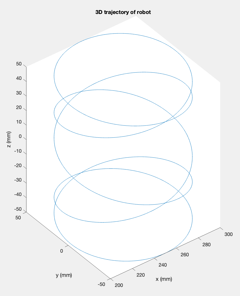
To understand the trajectory of the robot, we first plot it in 3D:

output = readmatrix("output.csv");
x = output(:, 1);
y = output(:, 2);
z = output(:, 3);
t = output(:, 4);
t_start = t(1);
t_end = t(end);
 
subplot(1,2,1);
plot3(x,y,z);
title("3D trajectory of robot")
xlabel("x (mm)");
ylabel("y (mm)");
zlabel("z (mm)");

We can see that the the arm moves in a roughly circular fashion, but this does not provide much information other than that $x$ and $y$ are likely closely related to each other. Looking at the graph, they can be related in terms of a circle centered around $(250, 0)$ with radius of apprxomiately $50$ :

(x - 250)^{2} + y^{2} = 5 0^{2}

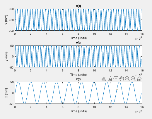
To learn more, we also plot $x (t), y (t), z (t)$ individually:

output = readmatrix("output.csv");
x = output(:, 1);
y = output(:, 2);
z = output(:, 3);
t = output(:, 4);
t_start = t(1);
t_end = t(end);
 
figure;
 
subplot(3,1,1);
plot(t, x);
title('x(t)');
xlabel('Time (units)');
ylabel('x (mm)');
 
subplot(3,1,2);
plot(t, y);
title('y(t)');
xlabel('Time (units)');
ylabel('y (mm)');
 
subplot(3,1,3);
plot(t, z);
title('z(t)');
xlabel('Time (units)');
ylabel('z (mm)');

From this, we see that the trajectory for each individual dimension appears to be periodic and resembles a sinusoid.

Curve fitting x(t)

Curve fitting y(t)

Curve fitting z(t)

Constraint Checking

Acceleration never exceeds $25 mm / s^{2}$ in any direction
Magnitude of acceleration never exceeds $50 mm / s^{2}$
Trajectory is infinitely differentiable

Part 2: Robot Kinematics

Forward Kinematics

Let’s summarize the given information/parameters:

Joint $J_{1}$ controls yaw (rotation around the $z$ -axis).
Joints $J_{2}$ and $J_{3}$ control pitch (rotation around the $y$ -axis).
$J_{2}$ and $J_{3}$ are perpendicular to each other when they are at $0$ , such that angle $J_{2}$ is measured from the $z$ -axis.
Link $L_{2}$ connects $J_{2}$ to $J_{3}$ and has a length of $135 mm$ .
Link $L_{3}$ connects $J_{3}$ to the end-effector and has a length of $147 mm$
A constant offset $O$ of $59.7 mm$ in the end-effector’s local frame in the positive $x$ direction.

J1 (xy direction)

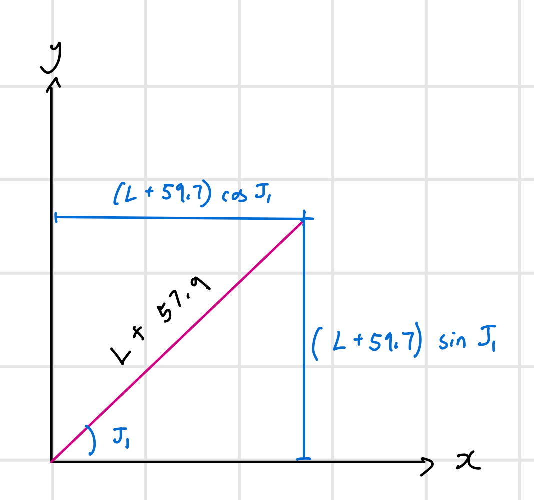
Since $J_{1}$ controls yaw (rotation around the $z$ -axis), it determines the direction of the arm in the $x y$ -plane. This can be stated in terms of the unit vector which strictly describes the direction of the arm:

u = ⟨ cos (J_{1}), sin (J_{1})⟩

However, we must also take into account the offset of $57.9 mm$ in the direction of $J_{1}$ . If we define the extended length of the arm (as viewed in the $x y$ plane) to be $L$ , the distance reached by the robot would be $L + 57.9$ . Combining this with the unit direction above, we can describe the $x$ and $y$ coordinates as:

(L + 57.9) u = ⟨(L + 57.9) cos J_{1}, (L + 57.9) sin J_{1}, 0 ⟩

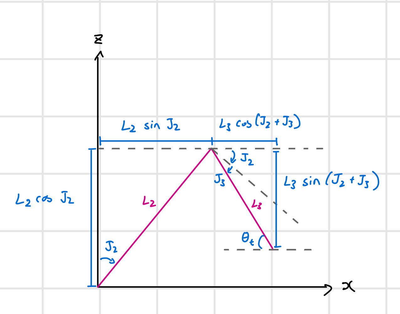
J2 and J3 (xy magnitude and height z)

Since $J_{2}$ and $J_{3}$ control pitch (rotation around $y$ -axis), they determine the magnitude of extended length $L$ in the $x y$ plane, as well as the height of the arm, $z$ . The effects of these joints can be determined in terms of the lengths of the links they control ( $L_{2}$ and $L_{3}$ ).

For link $L_{2}$ , we know that it has a length of $135 mm$ , and is controlled by $J_{2}$ which is constrained to $0° < J_{2} < 85°$ . Thus, we can describe its effect on $L$ and $z$ as:

L = 135 sin (J_{2}) + \dots z = 135 cos (J_{2}) + \dots

Due to the constraints on $J_{2}$ , we know that these effects always hold true as the sine and cosine of $J_{2}$ will always be positive and thus contribute to $L$ and $z$ . The ellipses indicate the terms derived below that describe the effect of link $L_{3}$ on $L$ and $z$ .

For link $L_{3}$ , we know that it has a length of $147 mm$ and is controlled by $J_{3}$ . Here, it is important that our coordinate system is defined correctly, as $L_{2}$ and $L_{3}$ form a right angle at zero position instead of being collinear. This relationship can be simplified by instead considering that the angle between $L_{2}$ and the horizontal is equal to $J_{2}$ when $J_{3}$ is zero.

We also need to consider changes to $L_{3}$ caused by changes in $J_{2}$ , such that the angle used for our trigonometric calculations of $L$ and $z$ is in fact $J_{2} + J_{3}$ . However, $J_{2} + J_{3}$ may be negative, which needs to be accounted for.

For $L$ , we use $cos$ because it takes on positive values on quadrants 1 and 4, because $L_{3}$ always contributes to $L$ due to the constraint on $J_{3}$ . Thus, we have:

L = 135 sin (J_{2}) + 147 cos (J_{2} + J_{3})

For $z$ , negative values of $J_{2} + J_{3}$ need to be added while positive values need to be subtracted from the height because the arm points down. Therefore, $- sin$ is used.

z = 135 cos (J_{2}) - 147 sin (J_{2} + J_{3})

Combining Equations

We combine the equations for $x$ and $y$ based on $J_{1}$ with the equations for $L$ and $z$ :

x y z = ((135 sin J_{2} + 147 cos (J_{2} + J_{3})) + 57.9) \cdot cos J_{1} = ((135 sin J_{2} + 147 cos (J_{2} + J_{3})) + 57.9) \cdot sin J_{1} = 135 cos (J_{2}) - 147 sin (J_{2} + J_{3})

Forearm angle determination

We are told that an increases in $J_{2}$ and $J_{3}$ angles result in the end-effector moving toward the table. When representing $Θ_{f}$ (forearm angle relative to horizontal) asa a function of $J_{2}$ and $J_{3}$ , we note that alternative interior angles must be equal to $J_{2} + J_{3}$ . This is shown in figure number. So we have:

Θ_{f} = J_{2} + J_{3}

Thus,

J_{3} = Θ_{f} - J_{2}

Validation

Plots

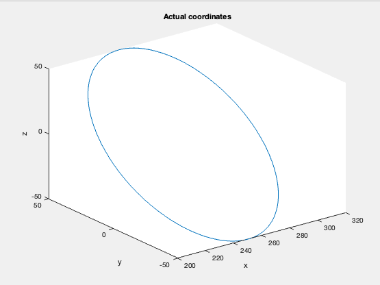
data = readmatrix("superCircleJoints.csv");
figure(1);
clf
x = data(:, 1);
y = data(:, 2);
z = data(:, 3);
j1 = data(:, 4);
j2 = data(:, 5);
theta_forearm = data(:, 6);
disp("Validation");
disp("Creating figures for actual and model plots");
plot3(x,y,z);
title("Actual coordinates");
xlabel("x");
ylabel("y");
zlabel("z");
 
%model
L = (147 .* cosd(theta_forearm)) + (135 .* sind(j2));
OFFSET = 59.7;
 
x_model = (L + OFFSET) .* cosd(j1);
y_model = (L + OFFSET) .* sind(j1);
z_model = (135 .* cosd(j2)) - (147 .* sind(theta_forearm));
 
figure(2);
clf
plot3(x_model, y_model, z_model);
title("Model coordinates");
xlabel("x");
ylabel("y");
zlabel("z");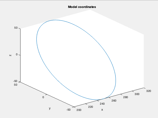

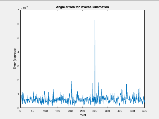
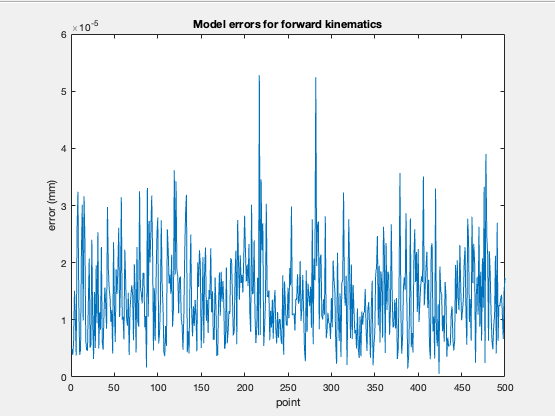
Error calculations:

% error calculations
x_errors = abs(x - x_model);
y_errors = abs(y - y_model);
z_errors = abs(z - z_model);
total_errors = hypot(x_errors, hypot(y_errors, z_errors));
total_max_e = max(total_errors);
total_min_e = min(total_errors);
disp(['max magnitude error ' num2str(total_max_e) ' mm'])
disp(['min magnitude error ' num2str(total_min_e) ' mm'])
rmse_total = sqrt(mean(total_errors.^2));
disp(['rmse total error ' num2str(rmse_total) ' mm'])
max magnitude error 5.2771e-05 mm
min magnitude error 5.6389e-07 mm
rmse total error 1.6182e-05 mm

Error plot:

Inverse Kinematics

To formulate an optimization

% calculating the constraints 
min_theta = -10; 
max_theta = 100; 
min_j2 = 0; 
max_j2 = 85; 
 
% assume angle constraint from diagram is for theta forearm 
min_j3 = min_theta - max_j2; 
max_j3 = max_theta - min_j2;
 
% functions must be defined at bottom of file 
function normal_distance = inverse_kinematics(p_r, p_d) 
	j1 = p_r(1); 
	j2 = p_r(2); 
	j3 = p_r(3); 
	
	x = p_d(1); 
	y = p_d(2); 
	z = p_d(3); 
	theta_forearm = j2 + j3; 
	l = (147 * cosd(theta_forearm)) + (135 * sind(j2)); 
	OFFSET = 59.7; 
	x_model = (l + OFFSET) * cosd(j1); 
	y_model = (l + OFFSET) * sind(j1); 
	z_model = (135 * cosd(j2)) - (147 * sind(theta_forearm)); 
	x_diff = abs(x_model - x); 
	y_diff = abs(y_model - y); 
	z_diff = abs(z_model - z); 
	normal_distance = hypot(x_diff, hypot(y_diff, z_diff)); 
end

/notes/

Recent

Gruebler's Equation

Kinematic Chain

MTE 309 A6

Serial Interfaces