Wasserstein GAN Loss

Wasserstein distance

We’ve seen that the GAN loss can be interpreted in terms of distances between probability distributions. In the original formulation, the gradient of this distance becomes zero when the generated samples are too easy to distinguish from the real examples. Thus, we aim to choose a distance metric with better properties.

The Wasserstein or earth mover’s distance (for discrete distributions) is the quantity of work required to transport the probability mass from one distribution to create the other. Here, “work” is defined as the mass multiplied by the distance moved. This makes the Wasserstein distance well-defined even when the distributions are disjoint and decreases smoothly as they become closer to one another.

Discrete (Earth mover’s distance)

Consider distributions $Pr(x=i)$ and $q(x=j)$ defined over $K$ bins. Assume there is a cost $C_{ij}$ associated with moving one unit of mass from bin $i$ in the first distribution to bin $j$ in the second. This cost might be the absolute difference $\left|i-j\right|$ between the indices. The amounts that are moved form the transport plan and are stored in the matrix $\mathbf{P}$.

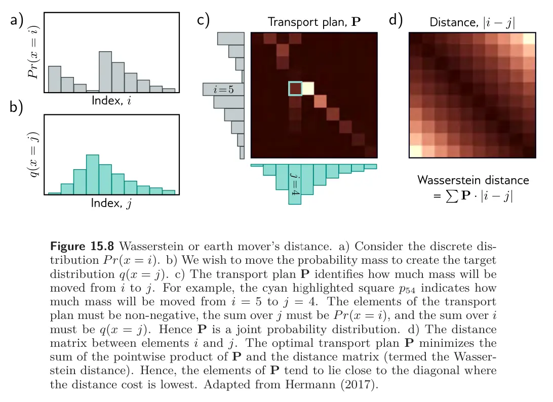
The Wasserstein distance is defined as:

$$D_w[Pr(x)\mid \mid q(x)]-\underset{\mathbf{P}}{\min }\left[\sum _{i,j}{P}_{ij}\cdot \left|i-j\right|\right]$$

subject to the constraints that:

• ${\sum }_j{P}_{ij}=Pr(x=i)$ – initial distribution of Pr(x)
• ${\sum }_i{P}_{ij}=q(x=j)$ – initial distribution of q(x)
• $P_{ij}\ge 0$ – non-negative masses

In other words, the Wasserstein distance is the solution to a constrained minimization problem that maps the masses of one distribution to the other. This is inconvenient, as we must solve this minimization problem over the elements $P_{ij}$ every time we want to compute the distance. Fortunately, this is a standard problem that is easily solved for small systems of equations. It’s a linear programming problem in its primal form:

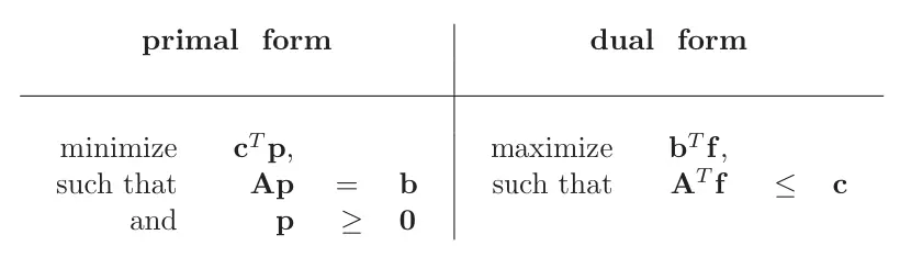
where $\mathbf{p}$ contains the vectorized elements $P_{ij}$ that determine the amount of mass moved, $\mathbf{c}$ contains the distance, $\mathbf{Ap}=\mathbf{b}$ contains the initial distribution constraints, and $\mathbf{p}\ge 0$ ensures the masses moved are non-negative.

As for all linear programming problems, there is an equivalent dual problem with the same solution. Here, we maximize with respect to a variable $\mathbf{f}$ that is applied to the initial distributions, subject to constraints that depend on the distances $\mathbf{c}$. The solution to this dual problem is:

$$D_w[Pr(x)\mid \mid q(x)]=\underset{\mathbf{f}}{\max }\left[\sum _{i}Pr(x=i)f_i-\sum _{j}q(x=j)f_j\right]$$

subject to the constraint that:

$$\left|f_{i+1}-f_i\right|<1$$

In other words, we optimize over a new set of variables $\{f_i\}$ where adjacent values cannot change by more than one.

Continuous

Translating the above results back to the continuous multi-dimensional domain, the equivalent of the primal form is:

$$D_w[Pr(\mathbf{x}),q(\mathbf{x})]=\underset{\pi [\bullet ,\bullet ]}{\min }\left[\int \int \pi ({\mathbf{x}}_1,{\mathbf{x}}_2)\cdot ||{\mathbf{x}}_1-{\mathbf{x}}_2||d{\mathbf{x}}_{1}d{\mathbf{x}}_2\right]$$

subject to similar constraints on the transport plan $\pi ({\mathbf{x}}_1,{\mathbf{x}}_2)$ representing the mass moved from position ${\mathbf{x}}_1$ to ${\mathbf{x}}_2$.

The equivalent of the dual form is:

$$D_w[Pr(\mathbf{x}),q(\mathbf{x})]=\underset{f[\mathbf{x}]}{\max }\left[\int Pr(\mathbf{x})f[\mathbf{x}]d\mathbf{x}-\int q(\mathbf{x})f[\mathbf{x}]d\mathbf{x}\right]$$

subject to the constraint the the Lipschitz constant of the function $f[\mathbf{x}]$ is less than one (the absolute gradient of the function is less than one)..

Wasserstein GAN loss

In the context of neural networks, we maximize over the space of functions $f[x]$ by optimizing the parameters $\varphi$ in a neural network $f[x,\varphi ]$, and we approximate these integrals using generated samples ${\mathbf{x}}_i^{\ast }$ and real examples ${\mathbf{x}}_i$:

$$\begin{array}{rl}L[\varphi ]& =\sum _{j}f[x_j^{\ast },\varphi ]-\sum _{i}f[x_i,\varphi ]\\ & =\sum _{j}f[g[z_j,\theta ],\varphi ]-\sum _{i}f[x_i,\varphi ]\end{array}$$

where we must constrain the neural network discriminator $f[x_i,\varphi ]$ to have an absolute gradient norm of less than one at every position:

$$\left|\frac{\partial f[x,\varphi ]}{\partial x}\right|<1$$

One way to achieve this is to clip the discriminator weights to a small range (e.g., $\pm 0.01$). An alternative is the gradient penalty Wasserstein GAN (WGAN-GP), which adds a regularization term that increases as the gradient norm deviates from unity.

dl
Why does using a Wasserstein distance loss function make GAN training more stable?
?
Compared to the Jensen-Shannon divergence used in the original GAN loss function, Wasserstein distance is well-defined even when the real/synthetic distributions are disjoint and decreases smoothly as they become closer to one another.

+++