UDL Chapter 5 Problems

Problem 5.1

Show that the logistic sigmoid function $\text{sig}[z]$ becomes $0$ as $z\to -\infty$, is $0.5$ when $z=0$, and becomes $1$ when $z\to \infty$, where

$$\text{sig}[z]=\frac{1}{1+\exp [-z]}$$

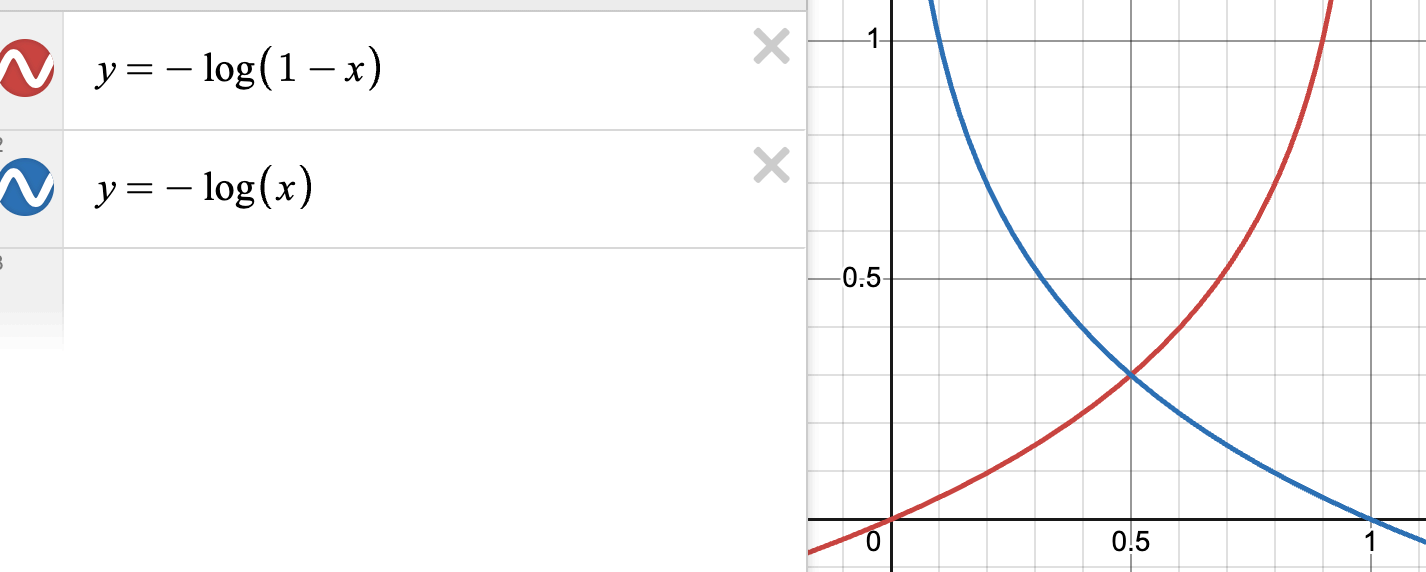
For $z\to -\infty$:

$$\underset{z\to -\infty }{\lim }\frac{1}{1+\exp [-z]}=\frac{1}{\infty }=0$$

For $z=0$:

$$\frac{1}{1+\exp [0]}=\frac{1}{1+1}=\frac{1}{2}=0.5$$

For $z\to \infty$:

$$\underset{z\to -\infty }{\lim }\frac{1}{1+\exp [-z]}=\frac{1}{1+0}=1$$

Problem 5.2

The loss $L$ for binary classification for a single training pair $\{\mathbf{x},y\}$ is

$$L=-(1-y)\log [1-\text{sig}[f[\mathbf{x},\varphi ]]]-y\log [\text{sig}[f[\mathbf{x},\varphi ]]]$$

Plot this loss as a function of the transformed output $\text{sig}[f[\mathbf{x},\varphi ]]\in [0,1]$ (i) when the training label $y=0$ and when (ii) when $y=1$.

When $y=0$, we just have $L=-1\log [1-\text{sig}[f[x,\varphi ]]]$. With $y=1$, we just have $L=-\log [\text{sig}[f[x,\varphi ]]]$:

Problem 5.3

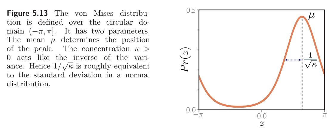
Suppose we want to build a model that predicts the direction $y$ in radians of the prevailing wind based on local measurements of barometric pressure $\mathbf{x}$. A suitable distribution over circular domains is the von Mises distribution:

$$Pr(y|\mu ,\kappa )=\frac{\exp [\kappa \cos [y-\mu ]]}{2\pi \cdot {\text{Bessel}}_0[\kappa ]}$$

• $\mu$ is a measure of the mean direction

• $\kappa$ is a measure of concentration (i.e. inverse of variance)

• The term ${\text{Bessel}}_0(\kappa )$ is a modified Bessel function of the first kind of order $0$.

  Use the loss function recipe to develop a loss function for learning the parameter $\mu$ of a model $f[\mathbf{x},\varphi ]$ to predict the most likely wind direction. Your solution should treat the concentration $\kappa$ as a constant. How would you perform inference?

We set $\mu =f[{\mathbf{x}}_i,\varphi ]$, so

$$Pr(y_i|f[x_i,\varphi ])=\frac{\exp [\kappa \cos [y-f[{\mathbf{x}}_i,\varphi ]]]}{2\pi \cdot {\text{Bessel}}_0[\kappa ]}$$

Then the negative log-likelihood loss function is

$$\begin{array}{rl}L& =-\sum _{i=1}^I\log \left(\frac{\exp [\kappa \cos [y-f[{\mathbf{x}}_i,\varphi ]]]}{2\pi \cdot {\text{Bessel}}_0[\kappa ]}\right)\\ & =-\sum _{i=1}^I[\kappa \cos [y-f[{\mathbf{x}}_i,\varphi ]]]-(\log (2\pi )+\log ({\text{Bessel}}_0[\kappa ]))\\ & =-\sum _{i=1}^I\cos [y-f[{\mathbf{x}}_i,\varphi ]]\end{array}$$

To perform inference we just take the maximum of the distribution (which is just the predicted parameter $\mu$). This might be out of the range $[-\pi ,\pi ]$, in which case we would add/remove multiples of $2\pi$ until it is in the right range.

Problem 5.4

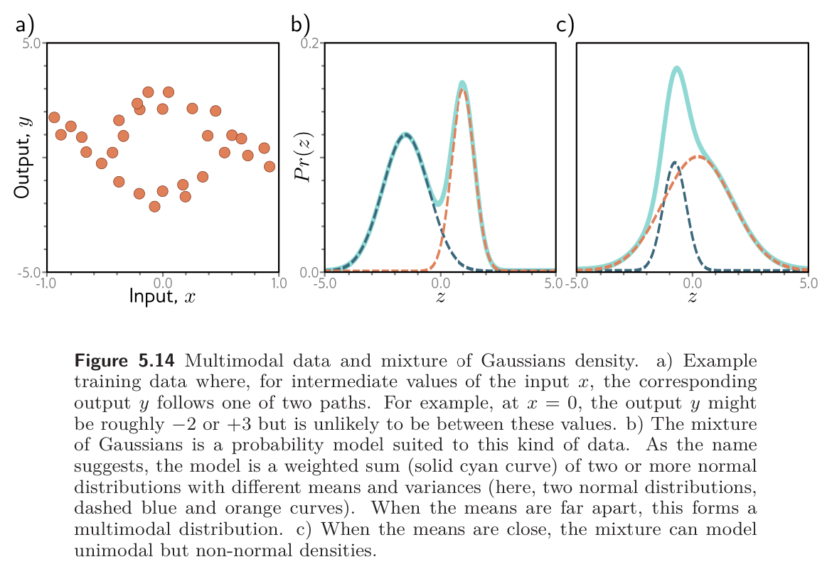
Sometimes, the outputs for input $\mathbf{x}$ are multimodal; there is more than one valid prediction for a given input. Here, we might use a sum of normal components as the distribution over the output. This is known as a mixture of Gaussians model. For example, a mixture of two Gaussians has parameters $\theta =\{\lambda ,{\mu }_1,{\sigma }_1^2,{\mu }_2,{\sigma }_2^2\}$:

$$Pr(y|\lambda ,{\mu }_1,{\mu }_2,{\sigma }_1^2,{\sigma }_2^2)=\frac{\lambda }{\sqrt{2\pi {\sigma }_1^2}}\exp \left[-\frac{(y-{\mu }_1{)}^2}{2{\sigma }_1^2}\right]+\frac{1-\lambda }{\sqrt{2\pi {\sigma }_2^2}}\exp \left[\frac{-(y-{\mu }_2{)}^2}{2{\sigma }_2^2}\right]$$

where $\lambda \in [0,1]$ controls the relative weight of the two components, which have means ${\mu }_1,{\mu }_2$ and variances ${\sigma }_1^2,{\sigma }_2^2$, respectively. This model can represent a distribution with two peaks or a distribution with one peak but a more complex shape.

Use the loss function recipe to construct a loss function for training a model $\mathbf{f}[x,\varphi ]$ that takes input $x$, has parameters $\varphi$, and predicts a mixture of two Gaussians. The loss should be based on $I$ training data pairs $\{x_i,y_i\}$. What problems do you foresee when performing inference?

Let:

• $\lambda =\text{sig}[{\mathbf{f}}_1[{\mathbf{x}}_i,\varphi ]]$
  • Use sigmoid to enforce $\lambda \in [0,1]$.
• ${\mu }_1={\mathbf{f}}_2[{\mathbf{x}}_i,\varphi ]$
• ${\sigma }_1={\mathbf{f}}_3[{\mathbf{x}}_i,\varphi ]$
• ${\mu }_2={\mathbf{f}}_4[{\mathbf{x}}_i,\varphi ]$
• ${\sigma }_2={\mathbf{f}}_5[{\mathbf{x}}_i,\varphi ]$

Then the loss is

$$L=-\sum _{i=1}^I\log \left[\frac{\text{sig}[{\mathbf{f}}_1[{\mathbf{x}}_i,\varphi ]]}{\sqrt{2\pi {\mathbf{f}}_3[{\mathbf{x}}_i,\varphi {]}^2}}\exp \left[\frac{-(y-{\mathbf{f}}_2[{\mathbf{x}}_i,\varphi ]{)}^2}{2{\mathbf{f}}_3[{\mathbf{x}}_i,\varphi {]}^2}\right]+\frac{1-\text{sig}[{\mathbf{f}}_1[{\mathbf{x}}_i,\varphi ]]}{\sqrt{2\pi {\mathbf{f}}_5[{\mathbf{x}}_i,\varphi {]}^2}}\exp \left[\frac{-(y-{\mathbf{f}}_4[{\mathbf{x}}_i,\varphi ]{)}^2}{2{\mathbf{f}}_5[{\mathbf{x}}_i,\varphi {]}^2}\right]\right]$$

Inference is a bit trickier in this case since there is no simple closed form for the mode of this distribution.

• MACP: How many modes can a Gaussian mixture have?

Problem 5.5

Consider extending the model from problem 5.3 to predict the wind direction using a mixture of two von Mises distributions. Write an expression for the likelihood $Pr(y|\theta )$ for this model. How many outputs will the network produce?

Each von Mises distribution is parametrized by $\mu ,\kappa$. Thus, for a mixture of two von Mises distributions, the parameters will be

$$\theta =\{\lambda ,{\mu }_1,{\kappa }_1,{\mu }_2,{\kappa }_2\}$$

where $\lambda$ is the relative weight of the two distributions. The likelihood will then be:

$$Pr(y|\lambda ,{\mu }_1,{\kappa }_1,{\mu }_2,{\kappa }_2)=\lambda \frac{\exp [{\kappa }_1\cos [y-{\mu }_1]}{2\pi \cdot {\text{Bessel}}_0[{\kappa }_1]}+(1-\lambda )\frac{[\exp [{\kappa }_2\cos [y-{\mu }_2]]}{2\pi \cdot {\text{Bessel}}_0[{\kappa }_2]}$$

Like the mixture of Gaussians above, we would need five outputs, unless we consider ${\kappa }_1$ and ${\kappa }_2$ to be constants, in which case we would need 3.

Problem 5.6

Consider building a model to predict the number of pedestrians $y\in \{0,1,2,\dots \}$ that will pass a given point in the city in the next minute, based on data $\mathbf{x}$ that contains information about the time of the day, the longitude and latitude, and the type of neighborhood. A suitable distribution for modeling counts is the Poisson distribution. This has a single parameter $\lambda >0$ called the rate that represents the mean of the distribution. The distribution has probability distribution function:

$$Pr(y=k)=\frac{{\lambda }^k{e}^{-\lambda }}{k!}$$

Design a loss function for this model assuming we have access to $I$ training pairs $\{{\mathbf{x}}_{\mathbf{i}},y_i\}$.

We make the rate $\lambda$ the learned parameter such that $\lambda =f[{\mathbf{x}}_i,\varphi ]$. Then, we have

$$\begin{array}{r}Pr(y_i=k|f[x_i,\varphi ])=\frac{f[{\mathbf{x}}_{\mathbf{i}},\varphi {]}^k{e}^{-f[{\mathbf{x}}_i,\varphi ]}}{k!}\end{array}$$

The loss function based on negative log-likelihood is then

$$\begin{array}{rl}L& =-\sum _{i=1}^I\log \left[\frac{f[{\mathbf{x}}_{\mathbf{i}},\varphi {]}^k{e}^{-f[{\mathbf{x}}_i,\varphi ]}}{y_i!}\right]\\ & =-\sum _{i=1}^{I}k\log [f[{\mathbf{x}}_i,\varphi ]]-f[{\mathbf{x}}_i,\varphi ]-\log [y_i!]\end{array}$$

We can drop the last term above since it doesn’t depend on $\varphi$. Also, we often would want to add a function like $\lambda =\exp (f[{\mathbf{x}}_i,\varphi ])$ or $\lambda =|f[{\mathbf{x}}_i,\varphi ]|$ to enforce the condition that $\lambda >0$, similarly to how we used sigmoid/softmax to enforce $0<\mu <1$ before. $\exp$ is likely a better choice because it is differentiable.

Problem 5.7

Consider a multivariate regression problem where we predict ten outputs, so $\mathbf{y}\in {\mathbb{R}}^{10}$, and model each with an independent normal distribution where the means ${\mu }_d$ are predicted by the network, and variances ${\sigma }^2$ are constant. Write an expression for the likelihood $Pr(\mathbf{y}|\mathbf{f}[\mathbf{x},\varphi ])$. Show that minimizing the negative log-likelihood of this model is still equivalent to minimizing a sum of square terms if we don’t estimate the variance ${\sigma }^2$.

Each probability likelihood is given by

$$Pr(y_{id}|f[{\mathbf{x}}_i,\varphi ])=\frac{1}{\sqrt{2\pi {\sigma }^2}}\exp \left[-\frac{(y_{id}-{\mu }_d{)}^2}{2{\sigma }^2}\right]$$

We try to learn parameters to predict each mean, such that ${\mu }_d={\mathbf{f}}_d[{\mathbf{x}}_{\mathbf{i}},\varphi ]$.

Then, the overall joint likelihood is given by

$$Pr({\mathbf{y}}_i\mid \mathbf{f}[{\mathbf{x}}_i,\varphi ])=\prod _{d=1}^{10}\frac{1}{\sqrt{2\pi {\sigma }^2}}\exp [-\frac{(y_{id}-f_d[{\mathbf{x}}_i,\varphi ]{)}^2}{2{\sigma }^2}].$$

Then:

$$\begin{array}{rl}L[\varphi ]& =-\sum _{i=1}^I\log [Pr({\mathbf{y}}_i|\mathbf{f}[{\mathbf{x}}_i,\varphi ])]\\ & =-\sum _{i=1}^I\sum _{d=1}^{10}\log [Pr(y_{id}|{\mathbf{f}}_d[{\mathbf{x}}_i,\varphi ])]\\ & =-\sum _{i=1}^I\sum _{d=1}^{10}\log \frac{1}{\sqrt{2\pi {\sigma }^2}}\exp \left[-\frac{(y_{id}-{\mathbf{f}}_d[{\mathbf{x}}_{\mathbf{i}},\varphi ]{)}^2}{2{\sigma }^2}\right]\end{array}$$

Then, following the derivation we did for least squares, we just have

$$\begin{array}{r}\hat{\varphi }=\underset{\varphi }{\mathrm{argmin}}\left[\sum _{i=1}^I\sum _{d=1}^{10}(y_{id}-{\mathbf{f}}_d[{\mathbf{x}}_i,\varphi ]{)}^2\right]\end{array}$$

• The terms with no relation to $\varphi$ were discarded since they have no effect on the location of $\hat{\varphi }$

Problem 5.8

Construct a loss function for making multivariate predictions $\mathbf{y}\in {\mathbb{R}}^{D_o}$ based on independent normal distributions with different variances ${\sigma }_d^2$ for each dimension. Assume a heteroscedastic model so that both the means ${\mu }_d$ and the variances ${\sigma }_d^2$ vary as a function of the data.

Let:

• ${\mu }_d={\mathbf{f}}_{1d}[{\mathbf{x}}_i,\varphi ]$
• ${\sigma }_d^2={\mathbf{f}}_{2d}[{\mathbf{x}}_i,\varphi ]$

Then the loss function is:

$$L=-\sum _{i=1}^I\log \left[\prod _{d=1}^{D_o}\frac{1}{\sqrt{2\pi {\mathbf{f}}_{2d}[{\mathbf{x}}_i,\varphi {]}^2}}\exp \left[-\frac{(y_{id}-{\mathbf{f}}_{1d}[{\mathbf{x}}_i,\varphi ])}{2{\mathbf{f}}_{2d}[{\mathbf{x}}_i,\varphi {]}^2}\right]\right]$$

We can do negative log-likelihood on the inside term too:

$$\begin{array}{rl}L& =-\sum _{i=1}^I\sum _{d=1}^{D_o}\log \left[\frac{1}{\sqrt{2\pi {\mathbf{f}}_{2d}[{\mathbf{x}}_i,\varphi {]}^2}}\exp \left[-\frac{(y_{id}-{\mathbf{f}}_{1d}[{\mathbf{x}}_i,\varphi ]{)}^2}{2{\mathbf{f}}_{2d}[{\mathbf{x}}_i,\varphi {]}^2}\right]\right]\end{array}$$

Taking the log of the product inside:

$$\begin{array}{rl}L& =\sum _{i=1}^I\sum _{d=1}^{D_o}\left\{\frac{1}{2}\log \right(2\pi {\mathbf{f}}_{2d}[{\mathbf{x}}_i,\varphi {]}^2)+\frac{(y_{id}-{\mathbf{f}}_{1d}[{\mathbf{x}}_i,\varphi ]{)}^2}{2{\mathbf{f}}_{2d}[{\mathbf{x}}_i,\varphi {]}^2}\}\end{array}$$

Problem 5.9

Consider a multivariate regression problem in which we predict the height of a person in meters and their weight in kilos from data $\mathbf{x}$. Here, the units take quite different ranges. What problems do you see this causing? Propose two solutions to these problems.

The values for weight in kilos (50-100 range) are going to be much higher than for height in meters (1-2m) range. Using least squares, the loss will focus much more on weight than height.

Possible solutions:

• Rescale/normalize outputs so they have the same standard deviation, build the model the predict the normalized outputs, and scale them back after inference
• Learn a separate variance for the two dimensions so that the model can automatically take care of this. This can be done in either a homoscedastic or heteroscedastic way.

Problem 5.10

Extend the model from problem 5.3 to predict both the wind direction and the wind speed and define the associated loss function.

Direction uses von Mises distribution in 5.3:

$$Pr(y|\mu ,\kappa )=\frac{\exp [\kappa \cos [y-\mu ]]}{2\pi \cdot {\text{Bessel}}_0[\kappa ]}$$

which results in a negative log-likelihood loss function of

$$L_{\text{direction}}=-\sum _{i=1}^I\cos [y-f_1[{\mathbf{x}}_i,\varphi ]]$$

For windspeed, we can use a Weibull distribution:

$$Pr(v|k,\lambda )=\frac{k}{\lambda }(\frac{v}{\lambda }{)}^{k-1}\exp [-(v/\lambda {)}^k]$$

where $k$ is a shape parameter and $\lambda$ is a scale parameter.

Using negative log likelihood on the Weibull distribution gives us

$$\begin{array}{rl}{L}_{\text{speed}}& =-\sum _{i=1}^I\log \left[\frac{k}{{\lambda }_i}{\left(\frac{v_i}{{\lambda }_i}\right)}^{k-1}\exp \left(-{\left(\frac{v_i}{{\lambda }_i}\right)}^k\right)\right]\\ & =-\sum _{i=1}^I\left[\log k-\log {\lambda }_i+(k-1)\log \left(\frac{v_i}{{\lambda }_i}\right)-{\left(\frac{v_i}{{\lambda }_i}\right)}^k\right]\\ & =-\sum _{i=1}^I\left[\log k-\log {\lambda }_i+(k-1)(\log v_i-\log {\lambda }_i)-{\left(\frac{v_i}{{\lambda }_i}\right)}^k\right]\\ & =-\sum _{i=1}^I\left[\log k+(k-1)\log v_i-k\log {\lambda }_i-{\left(\frac{v_i}{{\lambda }_i}\right)}^k\right].\end{array}$$

We can learn both $\lambda$ and $k$, or fix $k$ and just learn $\lambda$. Let’s say we learn both and have $\lambda =f_2[{\mathbf{x}}_i,\varphi ]$ and $k=f_3[{\mathbf{x}}_i,\varphi ]$. Then the complete loss function is:

$$\begin{array}{rl}{L}_{\text{total}}=\sum _{i=1}^I[& -\cos (y_i-f_1[{\mathbf{x}}_i,\varphi ])-\log f_3[{\mathbf{x}}_i,\varphi ]-(f_3[{\mathbf{x}}_i,\varphi ]-1)\log v_i-f_3[{\mathbf{x}}_i,\varphi ]\log f_2[{\mathbf{x}}_i,\varphi ]-{\left(\frac{v_i}{f_2[{\mathbf{x}}_i,\varphi ]}\right)}^{f_3[{\mathbf{x}}_i,\varphi ]}]\end{array}$$