Residual Block

Residual or skip connections are shortcut branches in the computation graph that add the input of a layer or block to its output.

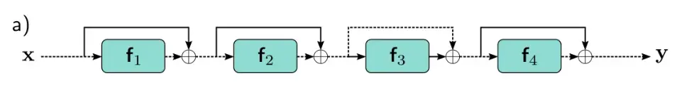
For example, the residual network below in Figure 11.4 computes:

$$\begin{array}{rl}{h}_1& =x+f_1[x,{\varphi }_1]\\ h_2& =h_1+f_2[h_1,{\varphi }_2]\\ h_3& =h_2+f_3[h_2,{\varphi }_3]\\ y& =h_3+f_4[h_3,{\varphi }_4]\end{array}$$

where the first term of every line is the residual connection. Thus, each layer $f_k$ computes an additive change to the current representation. This comes with the additional requirement that the input and output size must remain the same. Each additive computation of the input and processed output is called a residual block.

• $h_{k+1}=h_k+f_{k+1}[h_k]$ is a residual block.

We can re-write this as a single function by substituting the intermediate expressions:

$$\begin{array}{rl}y=x& +f_1[x]\\ & +f_2[x+f_1[x]]\\ & +f_3[x+f_1[x]+f_2[x+f_1[x]]]\\ & +f_4[x+f_1[x]+f_2[x+f_1[x]]+f_3[x+f_1[x]+f_2[x+f_2[x]]]]\end{array}$$

We can view this as unraveling the network, as shown in figure 11.4b below.

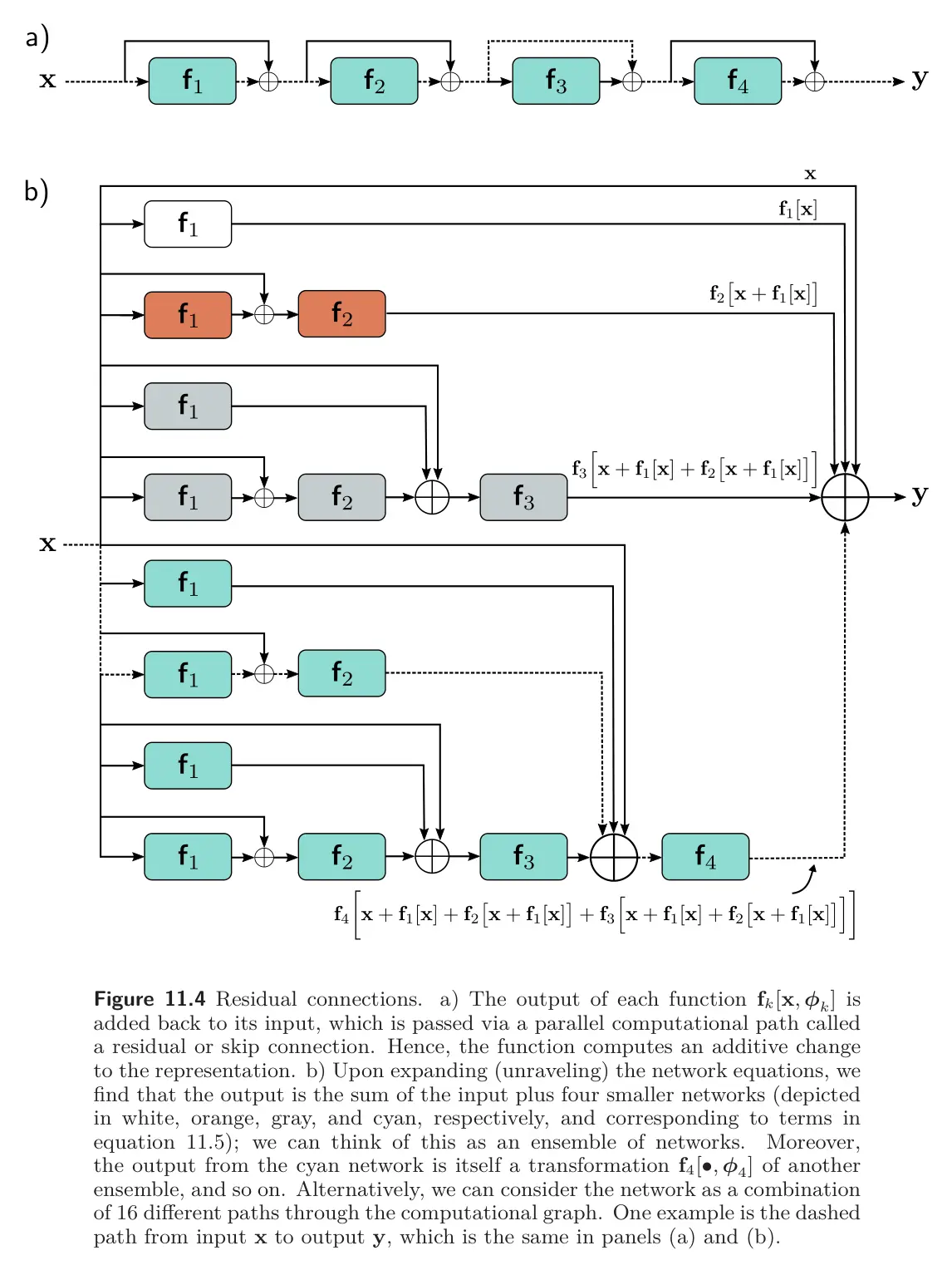
Ensembling view: From the unraveled equation/diagram, we could consider the final network to be a sum of the input and four smaller networks, each corresponding to a line of the equation.

Path view: Another complementary view is that the residual network creates 16 paths from the input to the output, each with differing transformations. For example, the first function occurs in 8/16 paths, including as a direct additive term (path length = 1). We can see this by considering the derivative $\frac{\partial y}{\partial f_1}$ and seeing that it consists of eight terms, one for each path.

$$\frac{\partial y}{\partial f_1}=I+\frac{\partial f_2}{\partial f_1}+\left(\frac{\partial f_3}{\partial f_1}+\frac{\partial f_3}{\partial f_2}\frac{\partial f_2}{\partial f_1}\right)+\left(\frac{\partial f_4}{\partial f_1}+\frac{\partial f_4}{\partial f_2}\frac{\partial f_2}{\partial f_1}+\frac{\partial f_4}{\partial f_3}\frac{\partial f_3}{\partial f_1}+\frac{\partial f_4}{\partial f_3}\frac{\partial f_3}{\partial f_2}\frac{\partial f_2}{\partial f_1}\right)$$

• The identity term corresponds to the direct addition term, showing that the parameters of the first layer $f_1[x,\varphi ]$ contribute directly to the changes in the network output $y$.
• The other terms are indirect contributions through other chains of derivatives of varying lengths.

In general, gradients through shorter paths will be better behaved. Since both the identity term and various short chains of derivatives will contribute to the derivatives of each layer, networks with residual links suffer less from shattered gradients, allowing us to increase the depth of the network significantly (by about double) without performance degradation. However, residual networks suffer from exploding gradients.

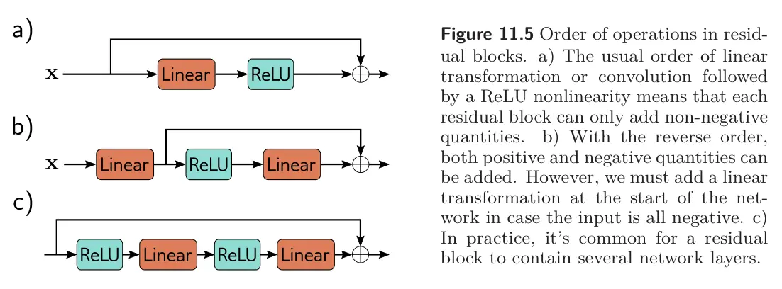
Order of operations in residual blocks

The layers $f[x]$, whether they are fully connected or convolutional, need to contain a nonlinear activation function, or the entire network will be linear. However, in a typical network layer, the ReLU function is at the end, so the output is non-negative. If we adopt this convention, then each residual block can only increase the input values.

Hence, we typically change the order of operations so that the activation function is applied first, followed by the linear transformation. Sometimes there may be several layers of processing within the residual block, but these usually terminate with a linear transformation.

Note that when we start these blocks with a ReLU operation, they will do nothing if the initial network is negative, since ReLU will clip the entire signal to zero. Thus, we typically start the network with a linear transformation.