A recurrent neural network allows us to process variable-length sequences. This is good for something like next-word prediction in a sentence.
RNNs’ key strength is their a hidden state, which acts as a memory of previous inputs. This allows the network to capture temporal dependencies and make information predictions based on past information.
- Increasing the size of (larger number of hidden units) enhances the ability to store and process long-term dependencies, but is more computationally expensive.
RNNs suffer from the Vanishing + Exploding Gradient Problem, making it difficult to learn dependencies over long timespans. More advanced architectures such as LSTM and GRU address these issues.
Vanilla RNN Formulation
RNNs process sequences by maintaining a hidden state that carries information from previous timesteps.
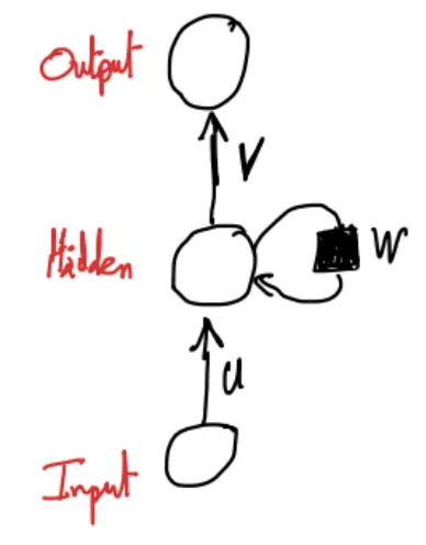
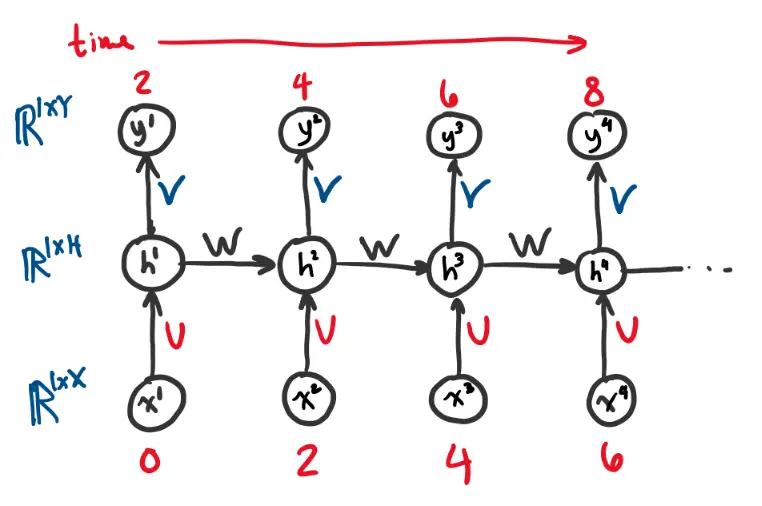
At each time step , the hidden state is updated using the previous hidden state and the current input.
- is the hidden state at time step
- is the input at time step
- is the input-to-hidden transformation weight matrix
- is the hidden-to-hidden transformation weight matrix (allows information to persist over time)
- is the bias term
- is a non-linear activation function
The output at each timestep is computed as
- is the output at time step
- is the hidden-to-output transformation weight matrix
- is the bias term
- The softmax function ensures that the output represents probabilities or conditional probabilities
Unrolled through time:
Backpropagation Through Time
The total loss function over a sequence of timesteps is computed as the sum of individual losses at each step:
- is the predicted output at each time step
- is the target/ground truth output at time step
- is the sequence length
- represents the loss function measuring the error between prediction and target at a given timestep. This could be a cross-entropy or MSE loss depending on the task.
- are weights for different timesteps
- The total loss is accumulated over all timesteps, ensuring that all predictions contribute to the optimization process.
Then, the training objective is to minimize the expected loss over the entire dataset:
After the forward pass, we can propagate the error gradients through the network.
Let us first consider the output pre-activation, .
With this we can get the gradient for the hidden-to-output weight matrix :
Hidden layers: Descending down to the hidden layer, it gets more interesting because each unrolled hidden layer depends on the one before it. So, we start at the final timestep and work our way back in time.
Define the “future-from-” loss as:
and consider .
The variables before timestep do not depend on the variables after ; depends on but not .
Therefore:
Thus, for the final hidden layer we have . This can be written as:
- Recall that
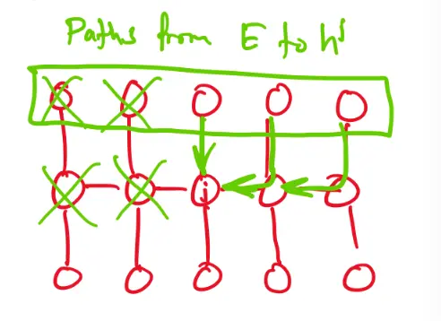
Note: All the backprop paths from to the variables must pass through for .
Suppose that we have already comptued . We we would like to compute :
Once you have , , you can compute the gradient with respect to the deeper weights and biases .
Vanishing/exploding gradient problem
We just saw that we have:
If we keep rolling this out recursively by writing out :
until we roll it out all the way:
This long multiplication chain causes instability.
Deep RNN
An RNN can be extended beyond a single layer by stacking multiple RNN layers vertically. This results in a deep RNN, which allows for hierarchical feature extraction across multiple levels of representation.
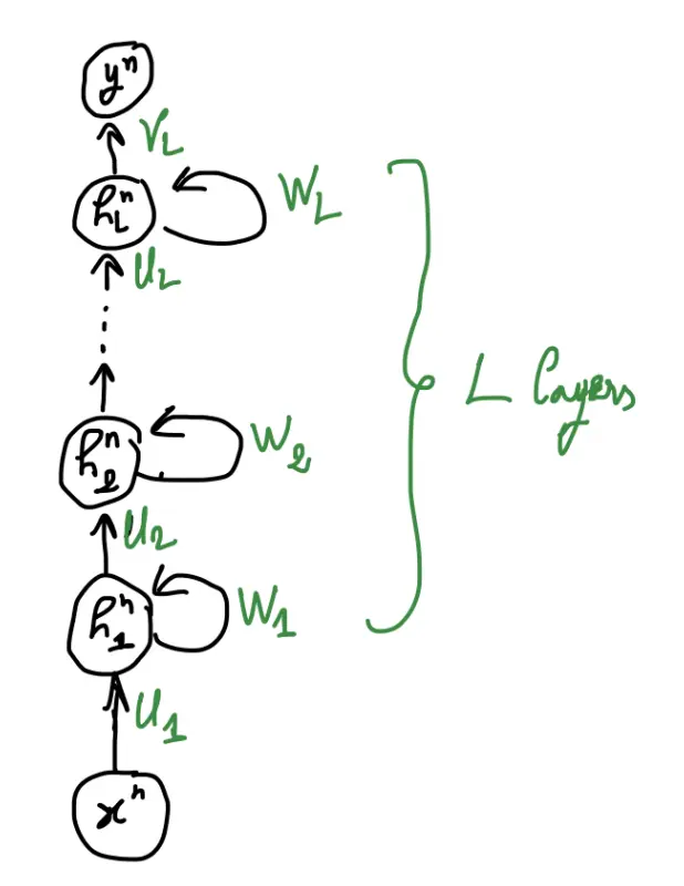
The key idea is that we have multiple layers of hidden states instead of a single hidden hidden state per timestep. Each layer processes information before passing it to the next layer.
- The input is first processed by the first RNN layer, generating a hidden state .
- Each subsequent layer receives the hidden state from the previous layer and computes a new hidden representation.
- The final layer produces the output .
The hidden states at each layer evolve as follows:
- is the hidden state at timestep in layer
- is the input-to-hidden weight matrix for layer
- is the recurrent weight matrix within layer
- is a non-linear activation function (e.g., tanh or ReLU)
- are vector biases
The final output is computed as where is the weight matrix from the last hidden layer to the output, and is a bias vector.