Long Term Short Memory

• Alex Colah’s blog on LSTMs

The benefit of an RNN is that it can accumulate a hidden state that encodes input over time. However, it can be hard to maintain information in its hidden state for a long time. Backpropagation through time becomes of exploding/vanishing gradients.

To combat this decay, the LSTM includes an additional “cell state” that persists from step to step. It does not pass through an activation function or get multiplied by the connection weights at each timestep.

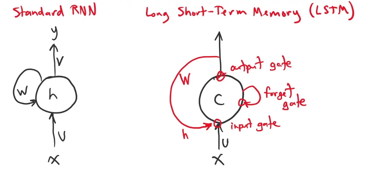
• $h$ and $x$ can increment $c$ (input)
• $h$ and $x$ can erase $c$ (forget)
• $h$ and $x$ can control the output of $c$ (output)

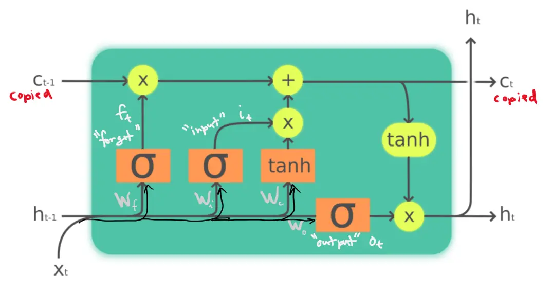
LSTM Formulation

Forget Gate

The forget gate determines whether to keep the current cell state or to flush it. It computes:

$$f_t=\sigma ([h_{t-1}{x}_t]W_f+b_f)$$

The sigmoid function outputs a value between 0 and 1. If 1, we completely persist. If 0, we completely forget. We’ll see how this works later.

Input Gate

The input gate determines how much of the input should be added to $c$. It computes:

$$i_t=\sigma ([h_{t-1}{x}_t]W_i+b_i)$$

Likewise, 1 = input, 0 = no input.

Cell state

A “candidate cell state” is calculated based on the past input hidden state.

$${\tilde{c}}_t=\tanh ([h_{t-1}{x}_t]W_c+b_c)$$

Then past and candidate cell states are combined to give the total cell state:

$$c_t=f_t\odot c_{t-1}+i_t\odot {\tilde{c}}_t$$

Output Gate

The output gate determines whether the cell state should influence the output. It computes:

$$o_t=\sigma ([h_{t-1}{x}_t]W_o+b_o)$$

where 1 = output and 0 = no output.

Output

Finally, we can compute the output as:

$$h_t=o_t\odot \tanh (c_t)$$

where $c_t$ can be written in one expression as

$$c_t=\underset{\text{Forget gate}}{\underbrace{\sigma (x_t{W}_f+b_f)}}{c}_{t-1}+\underset{\text{Input gate}}{\underbrace{\sigma (x_t{W}_i+b_i)}}\underset{\text{Candidate cell state}}{\underbrace{\tanh (x_t{W}_c+b_c)}}$$

Gradients

How does this make a difference with respect to solving the exploding/vanishing gradients problem?

We have:

$$c_t=f_t\odot c_{t-1}+i_t\odot {\tilde{c}}_{t-1}$$

How does ${\nabla }_{c_{t-1}}E$ depend on ${\nabla }_{c_t}E$? We hae:

$${\nabla }_{c_{t-1}}E={\nabla }_{c_t}E\odot f_t+\text{other stuff}$$

As long as $f$ is close to $1$, there is little decay of the gradient. Presumably $f$ is only close to $0$ when we actually want to forget. We don’t want to push gradient lower.

• Note that multiplying by $\sigma$ is different from multiplication by ${\sigma }^{\prime }$.

Essentially, the point is that the cell states evolve additively, When $f\approx 1$, the gradient can pass backward with little decay. This is much more stable than vanilla RNNs, where gradients are repeatedly multiplied by weight matrices and activation derivatives.