Linear Regression

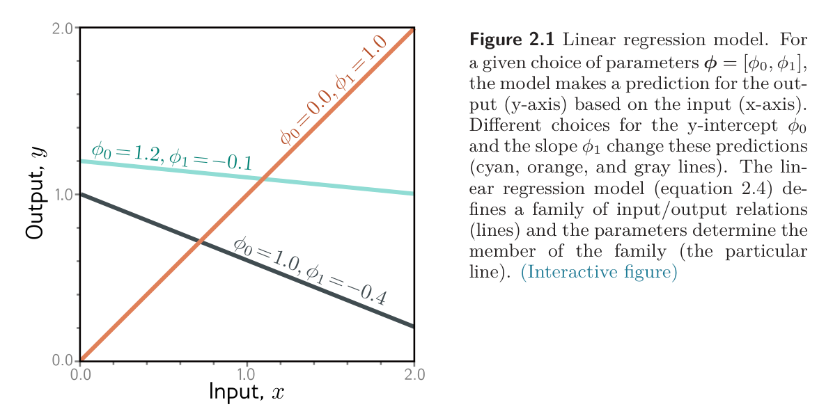
We can make the ideas of supervised learning more concrete with a simple example of regression. We consider a model $y=f[x,\varphi ]$ that predicts a single output $y$ from a single input $x$. A 1D linear regression model describes a straight line:

$$\begin{array}{rl}y& =f[x,\varphi ]\\ & ={\varphi }_0+{\varphi }_{1}x\end{array}$$

This model has two parameters $\varphi =[{\varphi }_0,{\varphi }_1]$, where ${\varphi }_0$ is the $y$-intercept of the line and ${\varphi }_1$ is the slope. Different choices for the intercept and the slope result in different relations, hence the model defines a family of possible input-output relations.

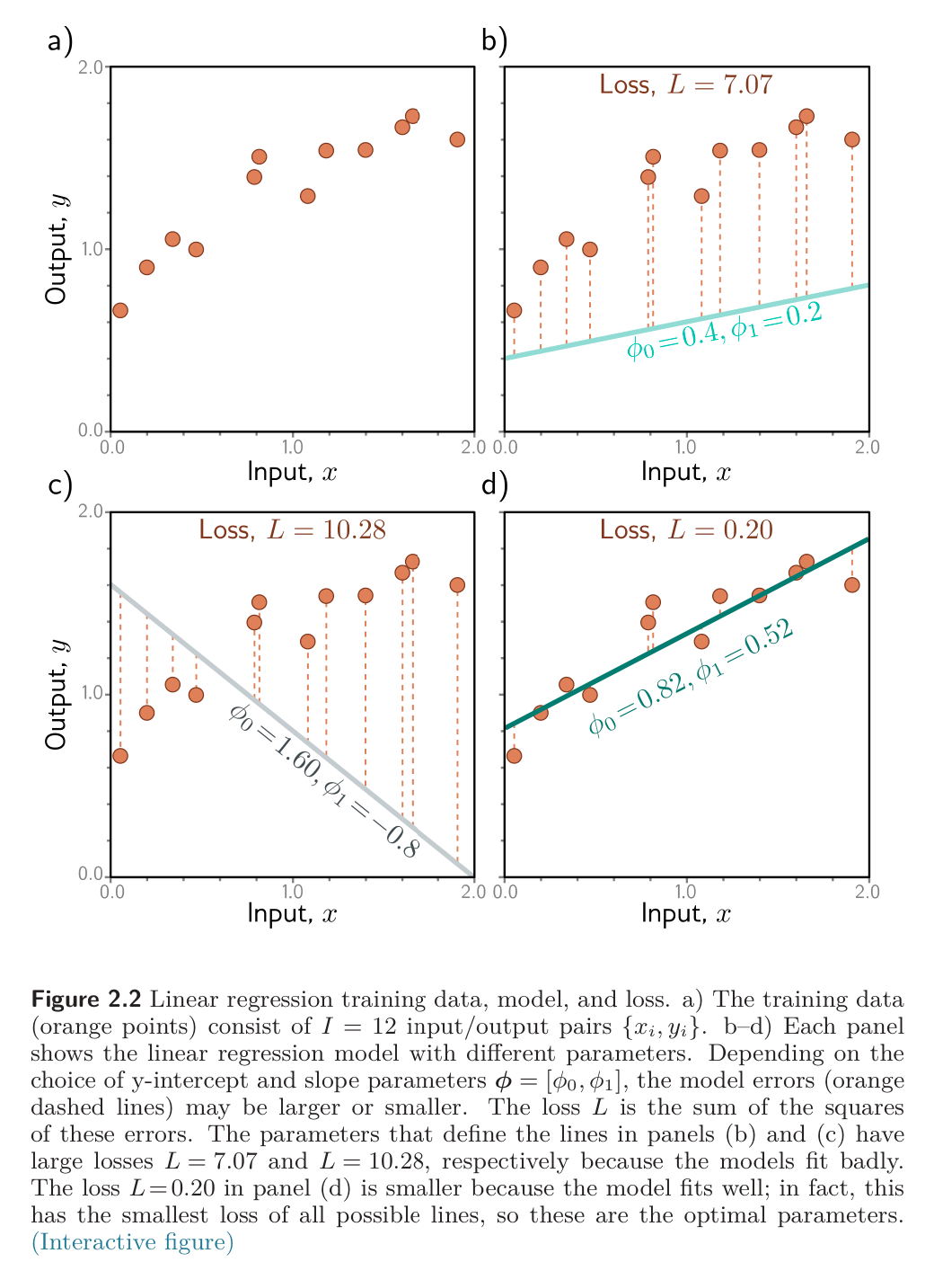
For this model, the training dataset consists of $I$ input/output pairs $\{x_i,y_i\}$. The mismatch between the model predictions $f[x_i,\varphi ]$ and the ground truth $y_i$. This loss is quantified using a sum of squares, over all $I$ training pairs:

$$\begin{array}{rl}L[\varphi ]& =\sum _{i=1}^I(f[x_i,\varphi ]-y_i{)}^2\\ & =\sum _{i=1}^I({\varphi }_0+{\varphi }_1{x}_i-y_i{)}^2\end{array}$$

This is called least-squares loss. The squaring operations means that the direction of the deviation (above/below the data) is unimportant.

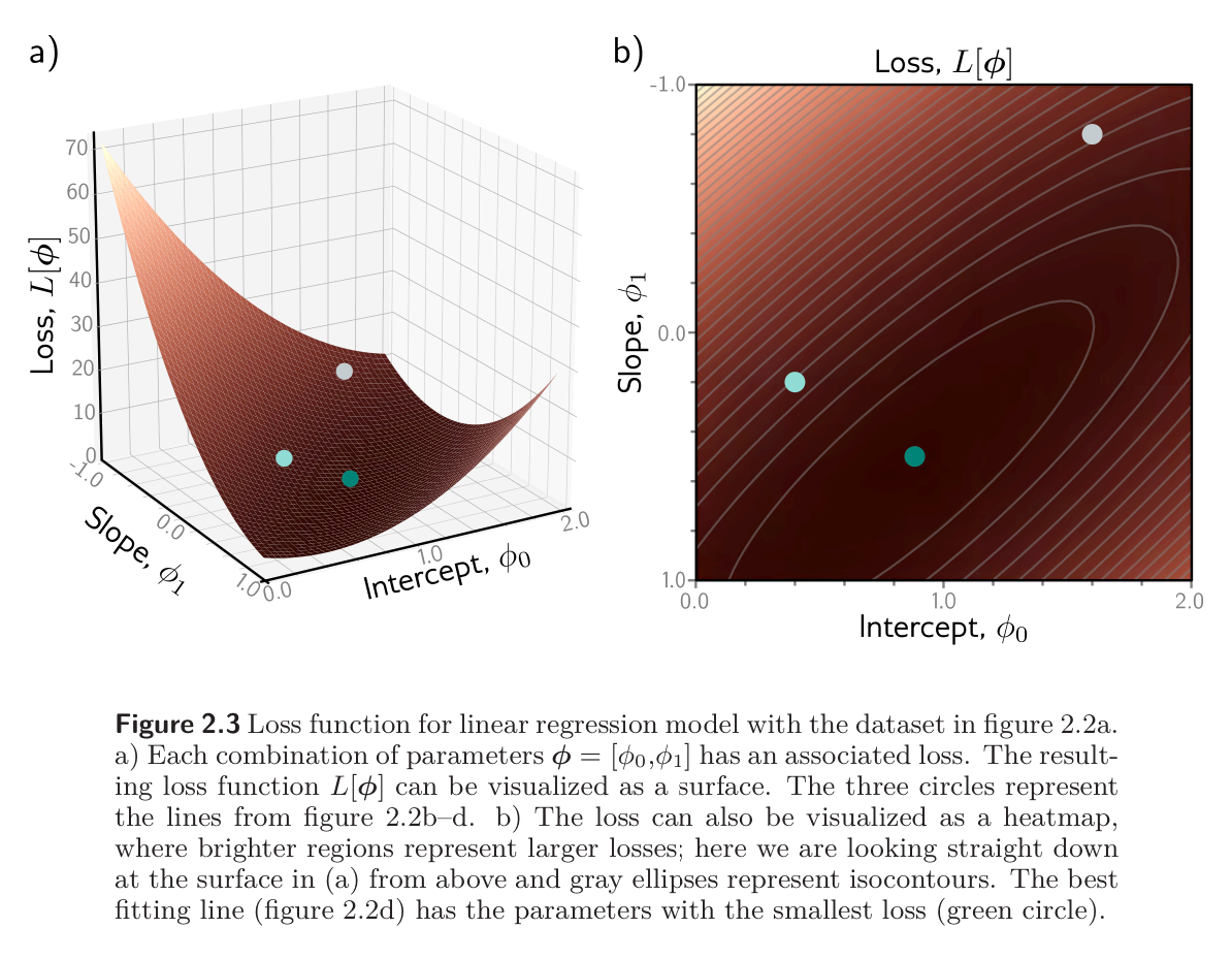
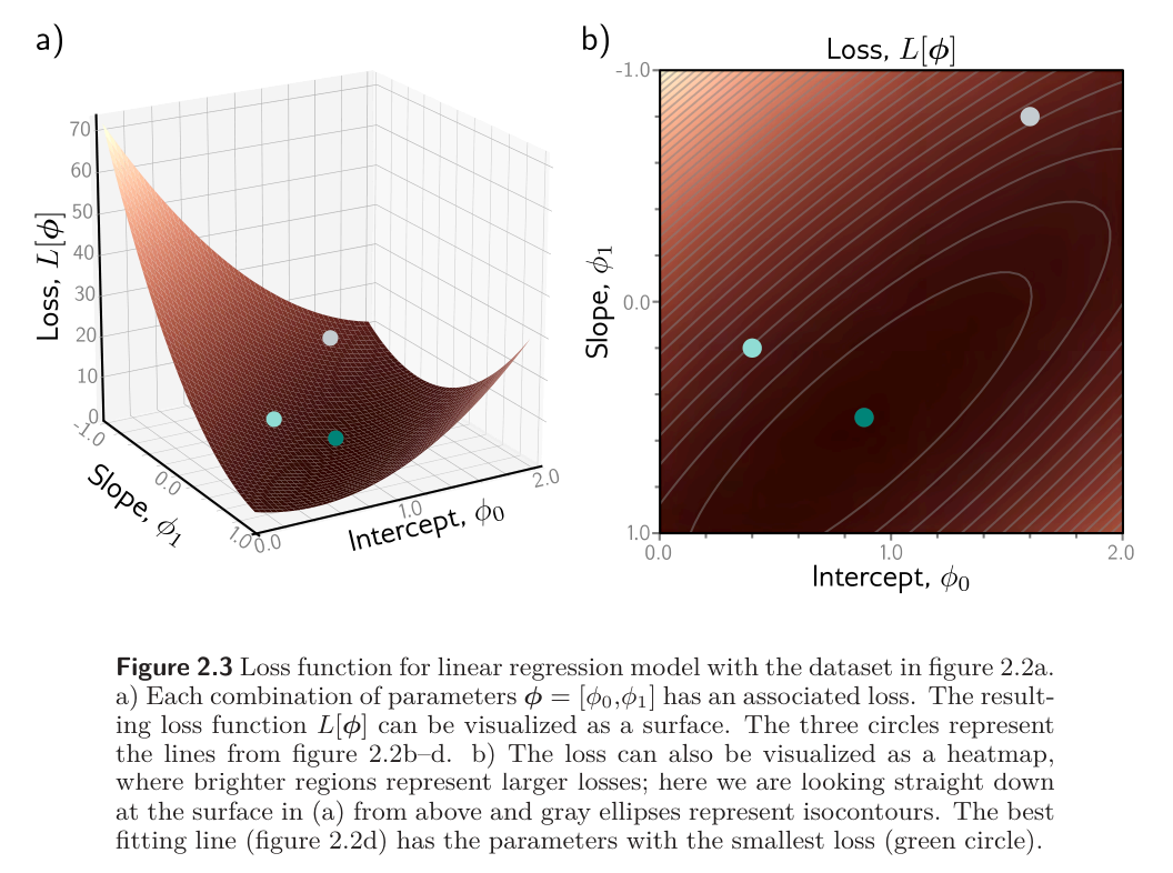
The goal of the training process is then to find the parameters $\hat{\varphi }$ that minimize this quantity:

$$\begin{array}{rl}\hat{\varphi }& =\underset{\varphi }{\mathrm{argmin}}[L[\varphi ]]\\ & =\underset{\varphi }{\mathrm{argmin}}\left[\sum _{i=1}^I(f[x_i,\varphi ]-y_i{)}^2\right]\\ & =\underset{\varphi }{\mathrm{argmin}}\left[\sum _{i=1}^I({\varphi }_0+{\varphi }_1{x}_i-y_i{)}^2\right]\end{array}$$

There are only two parameters, so we can calculate the loss for every combination of values and visualize the loss function as a surface. The “best” parameters are at the minimum of this surface.

For training and testing, the basic method is to choose the initial parameters randomly and then improve them by “walking down” the loss function until we reach the bottom. One way to do this is to measure the gradient of the surface at the current position and take a step in the direction that is most steeply downhill. Then we repeat this process until the gradient is flat and we can improve no further.

Having trained the model, we test it by computing the loss on a separate set of test data. This shows how well the training data generalizes.

• A simple model like a line might not be able to capture the true relationship between input and output. This is known as underfitting.
• Conversely, a very expressive model may describe statistical peculiarities of the training data that are atypical and lead to unusual predictions. This is known as overfitting.