Downsampling, upsampling, and changing the number of channels can be useful for working with 2D representations.
Downsampling
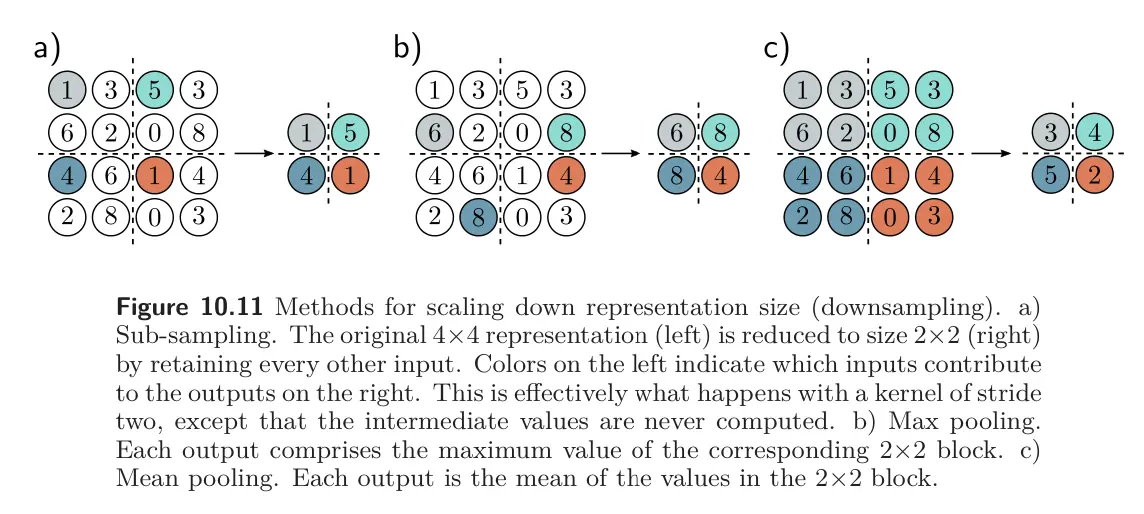
Let’s say we want to scale down by dimensions by a factor of 2. The easiest way to scale down is sub-sampling: sampling every other position. When we use a stride of two, we are effectively using this method simultaneously with the convolution operation.
Max pooling retains the maximum of the 2x2 input values. This induces some invariance to translation; if the input is shifted by one pixel, many of the maximum values will remain the same.
Mean pooling or average pooling averages the inputs.
For all approaches, we apply downsampling separately to each channel, so the output has half the width and height but the same number of channels.
Upsampling
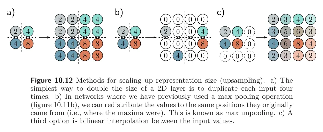
- The simplest way to scale up a network layer to double the resolution is to duplicate all the channels at each spatial position four times.
- Another way is max unpooling; this is used when we have previously used a max pooling operation for downsampling, and we distribute the values to the positions they originated from
- A third approach uses bilinear interpolation to fill in the missing values between the points where we have samples.
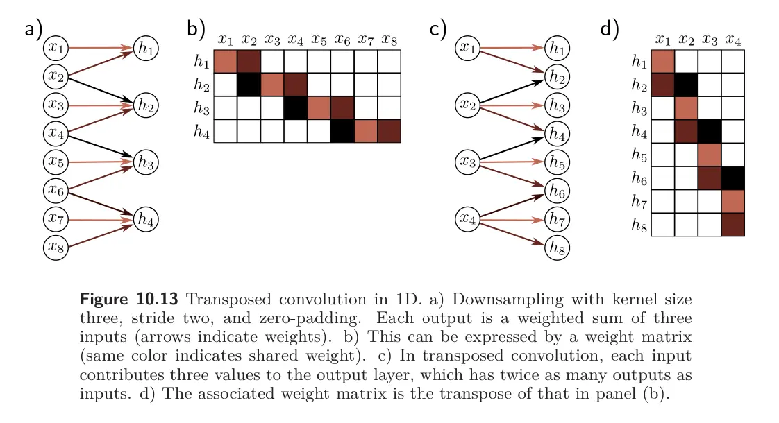
- A fourth approach is roughly analogous to downsampling using a stride of two. In that method, there were half as many outputs as inputs, and for kernel size 3, each output was a weighted sum of the three closest inputs. In transposed convolution, we reverse this. There are twice as many outputs as inputs, and each input contributes to three of the outputs. When we consider the associated weight matrix of this upsampling mechanism, we see that it is the transpose of the matrix for the downsampling mechanism.
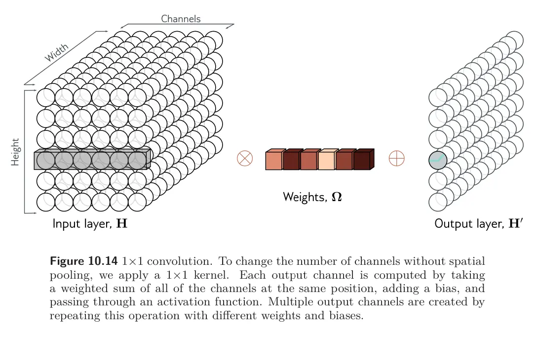
Changing the number of channels
Sometimes we want to change the number of channels between one hidden layer and the next without further spatial pooling. This is usually so we can combine the representation with another parallel computation (like a residual). To accomplish this, we apply a convolution with kernel size one. Each element of the output layer is computed by taking a weighted sum of all the channels at the same position. We can repeat this multiple with different weights to generate as many output channels as we need. The associated convolution weights have size , hence this is a convolution. Combined with a bias and activation function, this is equivalent to running the same fully connected network on the input channels at every position.