BatchNorm Backprop

BatchNorm introduces two parameters, $\gamma$ and $\delta$, which are used for scaling and shifting the normalized activations. These parameters are learned, which means we have to backpropagate through them.

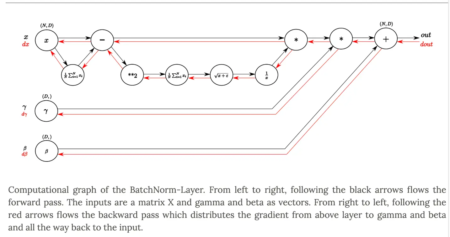
To see how this is done, we can consider the computational graph of batchnorm:

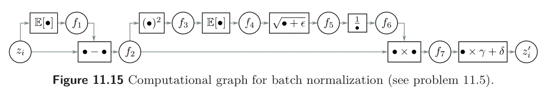
A vanilla implementation of the forward pass following the first version of the graph:

def batchnorm_forward(z, gamma, delta, eps=1e-5):
    B, D = z.shape
    assert gamma.shape == (D,)
    assert delta.shape == (D,)
 
    f1 = np.mean(z, axis=0, keepdims=True) #(1,D)
    f2 = z - f1 #(B,D)
    f3 = f2 ** 2 #(B,D)
    f4 = np.mean(f3, axis=0, keepdims=True) #(1,D)
    f5 = np.sqrt(f4 + eps) #(1,D)
    f6 = 1./f5 #(1,D)
    f7 = f2 * f6 #(B,D)   # normalized activations
    z_new = f7 * gamma + delta #(B,D)
    
    cache = (z, gamma, f1, f2, f3, f4, f5, f6, f7, eps)
 
    return z_new, cache

To do the backward pass, we go through the steps in reverse. Assume that we are given the gradient of the loss with respect to the batchnormed activations, dout.

def batchnorm_backward(dout, cache):
 
    # get intermediate values from cache
    z, gamma, f1, f2, f3, f4, f5, f6, f7, eps = cache 
    
    # get shapes from output
    B, D = dout.shape
    
    ddelta = np.sum(dout, axis=0) #(D,)
    dgamma = np.sum(dout * f7, axis=0) #(D,)
    df7 = dout * gamma #(B,D)
    df6 = np.sum(df7 * f2, axis=0, keepdims=True) #(1,D)
    df5 = df6 * (-1.0/(f5 ** 2)) #(1,D)
    df4 = df5 * (1.0/(2 * np.sqrt(f4+eps))) #(1,D)
        # can also be simplified to df5 * (1.0/(2 * f5)))
    df3 = np.ones_like(f3) * df4/B #(B,D)
 
    # two gradient paths for f2
    df2_fromf3 = df3 * 2 * f2
    df2_fromf7 = df7 * f6
    df2 = df2_fromf3 + df2_fromf7 #(B,D)
    
    df1 = -np.sum(df2, axis=0, keepdims=True) #(1,D)
    
    # two gradient paths for z
    dz_fromf2 = df2 #(B,D)
    dz_fromf1 = np.ones_like(z) * df1/B
    dz = dz_fromf2 + dz_fromf1
    
    return dz, dgamma, ddelta