Simulated Annealing

Simulated annealing is a trajectory search method inspired by the thermodynamic cooling of materials. A temperature parameter controls the randomness of motion, allowing us to converge from exploration to exploitation.

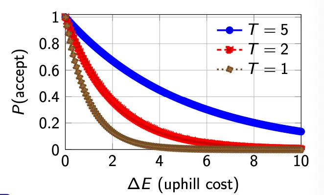
SA uses a probabilistic rule (Boltzmann acceptance probability):

$$P(\text{accept }{s}^{\prime })=\{\begin{array}{ll}1,& \Delta E\le 0\\ \exp (-\Delta E/T),& \Delta E>0\end{array}$$

where $E$ is our cost function. That is, we always accept improving moves, and sometimes accept non-improving moves.

The temperature parameter $T$ governs this:

• $T$ high → More exploration (accept more uphill moves)
• $T$ low → More exploitation (mostly greedy)

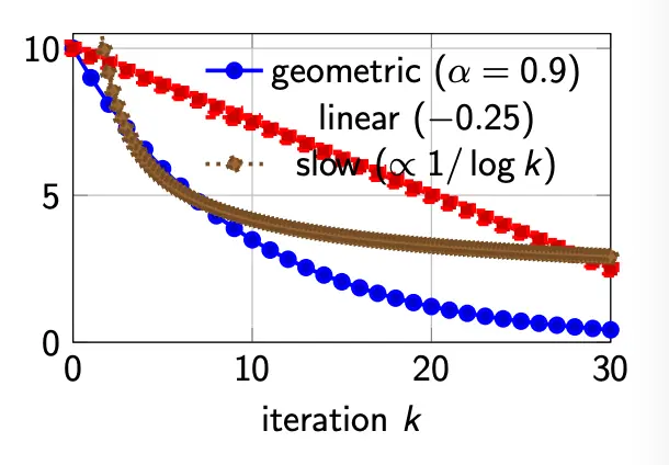
Cooling Schedules

$T$ is not held constant, but follows a schedule, such that we explore early and then exploit later. We don’t want a schedule that is too fast (basically becomes hill climbing early), or one that is too slow (wastes time wandering).

Common schedule:

• Geometric: $T_{k+1}=\alpha T_k$, where $\alpha \in (0,1)$.
  • This is a practical default.
• Linear: $T_{k+1}=T_k-\gamma$.
  • This is easy to reason about
• Very slow: $T_k\propto 1/\log (k)$.
  • This provides some theoretical guarantees but is often too slow.

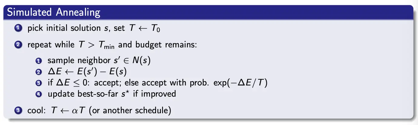
Pseudocode

Example

We aim to minimize energy $E(s)$. Let our current $E(s)=10$, with temperature $T=5$.

We take a random move in the neighborhood and sample a neighbor with $E(s^{\prime })=11$.

Then:

$$\Delta E=E(s^{\prime })-E(s)=11-10=1$$

and

$$P(\text{accept})=e^{-1/5}\approx 0.818$$

Thus, even the move is worse, it is likely accepted due to the high $T$. This enables barrier crossing early in the run.

For $\Delta E=1$, what is $P(\text{accept})$ for different temperatures?

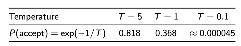
Thus, we see that cooling converts from exploration (many uphill moves allowed) to exploitation (almost greedy).

Practical Considerations

To make simulated annealing work better in practice, we do:

• Adaptive neighborhood control
• Reheating and strategic restarts:
  • Detect stagnation: no improvement over $K$ iterations
  • Increase temperature temporarily: $T\leftarrow \gamma T$, with $\gamma >1$
  • Allows escape from a deep local minima without discarding accumulatd structure
• Multiple trials per temperature level
  • Perform $L$ neighbor evaluations at each temperature $T$
  • Reduces sensitivity to unlucky single moves

Convergence Theory

The behavior of SA with constant temperature can be modeled using a Markov Chain. This is pretty intuitive – at a fixed $T$, SA defines a stochastic transition where the next state only depends on the current state, satisfying the Markov property.

It has been shown that under constant temperatures and as long as it’s possible to find a sequence of exchanges that will transform any solution to another with non-zero probability, the process converges, independent of the starting solution.

With non-constant temperature, we have a non-homogeneous Markov chain. This converges if the temperature is reduced to zero slowly with a specific logarithmic form (that very slow cooling schedule) and the number of iterations at each temperature is large (exponential in terms of size).

SA and Machine Learning

• Reinforcement Learning (RL) aims to maximize expected future reward. Rewards depend on sequences of past actions, not isolated decisions. The system evolves via a probabilistic state transition function driven by the current state and chosen action. Actions represent control decisions that affect both immediate reward and future system states. This coupling makes RL optimization highly non-trivial. Adaptive Simulated Annealing is used to optimize RL parameters, leading to improved control policies.
• Deep learning-enabled SA for topology optimization. Topology optimization is a high-dimensional, stochastic optimization problem requiring millions of expensive finite-element evaluations. The computational cost of classical SA becomes prohibitive for large-scale designs. A DNN is integrated with Generative Simulated Annealing (GSA) to approximate the objective function. GSA uses the DNN for fast evaluation, while newly generated solutions are used to continually retrain the DNN. The DNN–GSA loop converges to high-quality solutions with over two orders of magnitude reduction in computational cost.