Traditional population-based metaheuristics use random mutation and choose step sizes externally. The direction is also not explicitly modeled. Differential evolution uses differences between individuals to extract direction and scale from the population, generating solutions using this internal structure. Thus, instead of data variation, we use data-driven direction search.
GA recombines parent material, while DE constructs a directional perturbation using population differences. Thus, DE is more geometric than classical GA, and tends to be better suited for real-valued continuous optimization. ES uses Gaussian mutation with self-adaptation and step-size control; CMA-ES goes further by learning covariance structure. DE is simpler, with no explicit covariance matrix and no Gaussian assumption, uses pairwise population differences directly.
Walkthrough
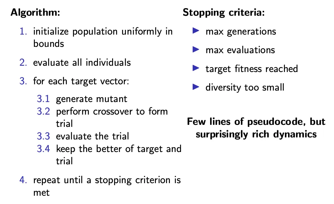
We maintain a population of candidate solutions:
- each is a point in the search space
- the population evolves over iterations
Then, we aim to improve each using information from other solutions.
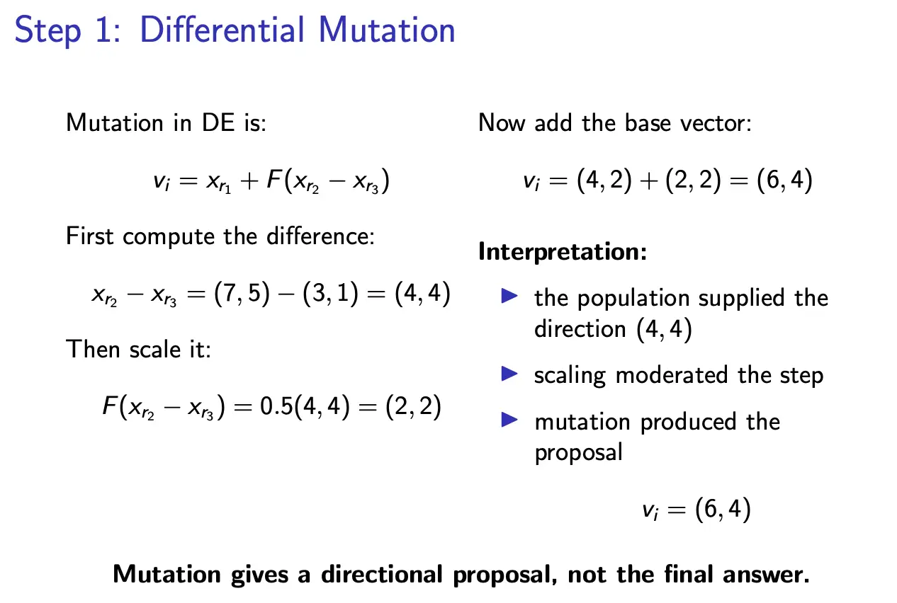
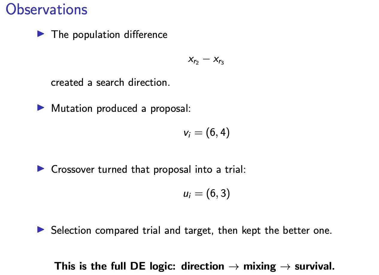
Step 1: Generating a direction and mutation
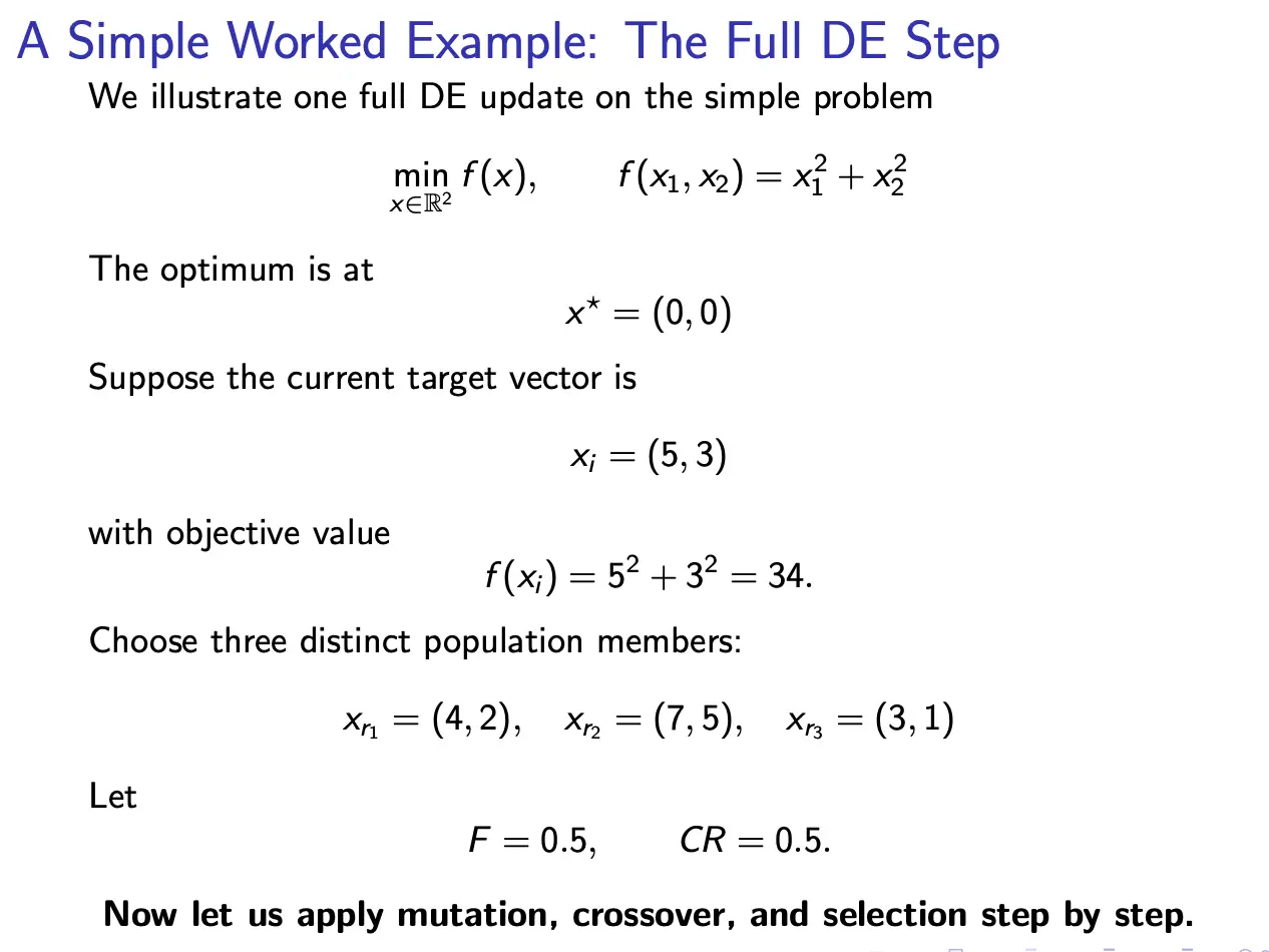
We pick three distinct solutions:
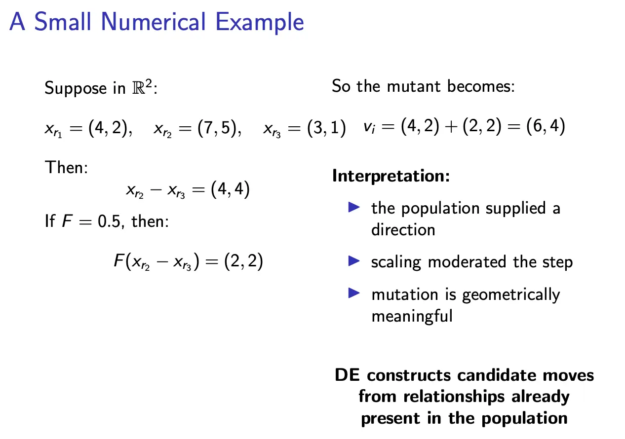
and form a direction vector:
We can then construct a new candidate:
where is a scaling factor.
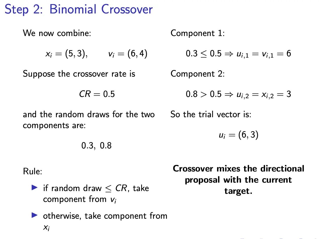
Step 2: Crossover
We now combine the original solution with the proposal . For exach component :
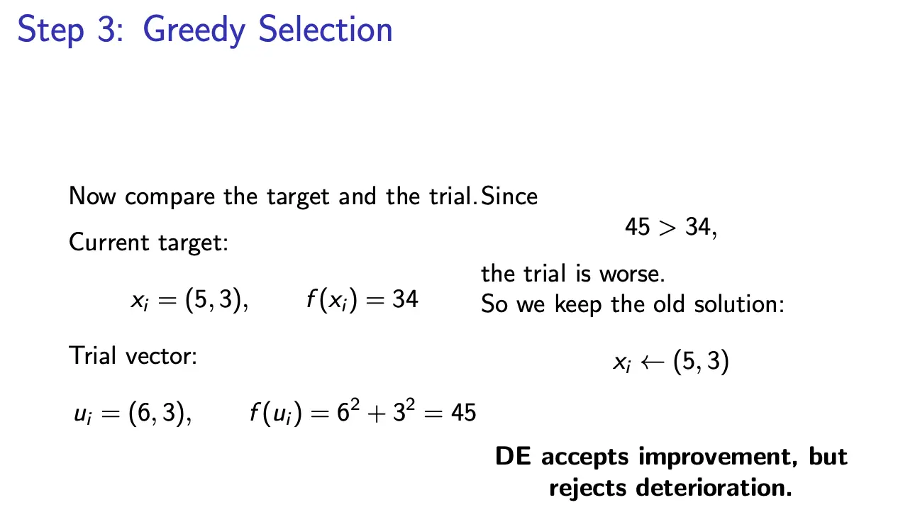
Step 3: Selection
We then compare the trial vector with the current solution :
Note: DE can generate infeasible trial vectors, so we often enforce some constraints like clipping to bounds.
Characteristics
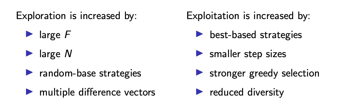
In DE, the step size comes from the population spread, and the direction comes from population differences. This leads to automatic scaling, and adaptive exploration vs. exploitation. And don’t have to deal with estimating gradients, covariance, or moving randomly.
The idea is that at any stage of the search, the population has a center and a spread. If two solutions are far apart, their difference encodes the scale, orientation, and diversity.
DE Strategies
The general notation for these strategy names is DE/base/num/cross.
- Base: where the mutation starts
- Num: how many difference vectors are used
- Cross: how recombination is done
DE/rand/1/bin
This is the canonical form we saw before, using random base vectors, with 1 difference vector, and binomial crossover. The mutation is:
Then, crossover builds , and selection compares with .
DE/best/1/bin
Now the mutation is given by:
such that the current best individual anchors the mutation. This gives faster convergence and stronger exploitation, but diversity may collapses sooner, with premature convergence being likely.
DE/current-to-best/1
Another common strategy is:
This combines attraction toward the current best, and a differential perturbation for diversity. Essentially, one term pulls toward exploitation, while another term injects exploratory motion.
Parameters
Scale factor
The scale factor controls the magnitude of differential mutation. If is small, we move cautiously, resulting in fine local search at the risk of stagnation. If is large, we take bold jumps, with stronger exploration, but at the risk of overshooting. Typically, we set .
Crossover rate
controls how much of the mutant enters the trial candidate. If CR is low, only a few components come from the mutant, preserving more of ; this results in conservative search. If CR is high, more mutant components survive, so search is more disruptive and exploration is stronger. Typically, we set .
Population size
Population size affects diversity, the sampling of difference directions, and computational cost. If is too large, we need to do a lot of evaluations, resulting in slower iteration and possibly redundant sampling. If is too small, we get weak diversity, poor directional information, and early stagnation. Rule of thumb: .
Cost
For each generation, each target vector produces one trial . Each trial requires one function evaluation. Thus, the total evaluations per generation is .
Objective evaluation is often the dominant cost; DE adds minimal overhead beyond evaluation. This is one of the upsides of DE; we are essentially trading sophistication for sampling efficiency.
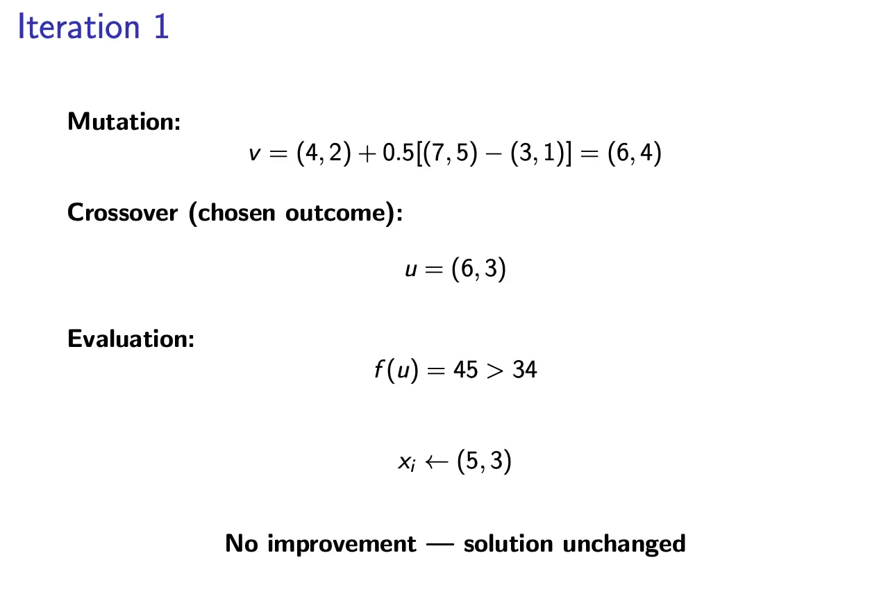
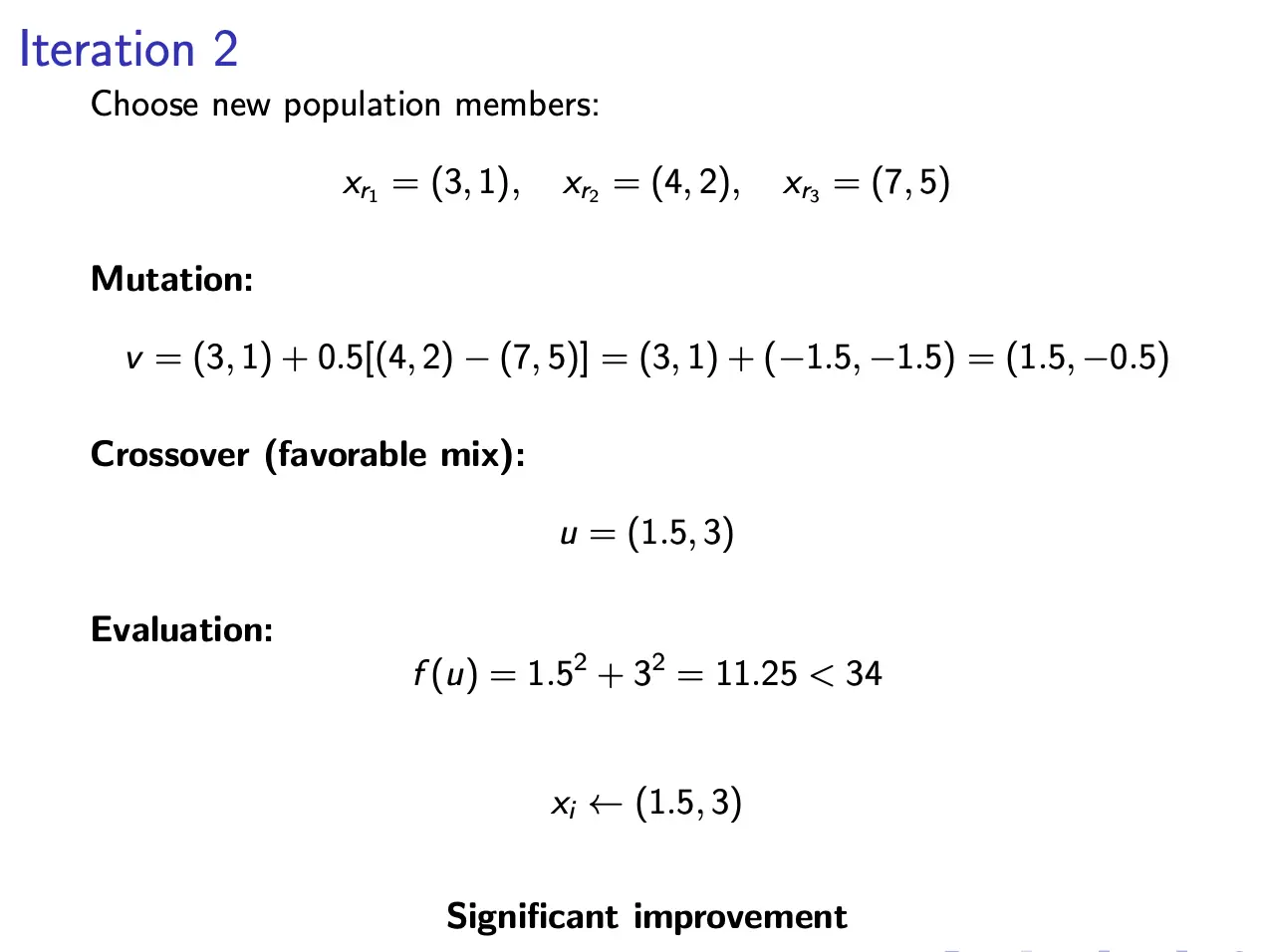
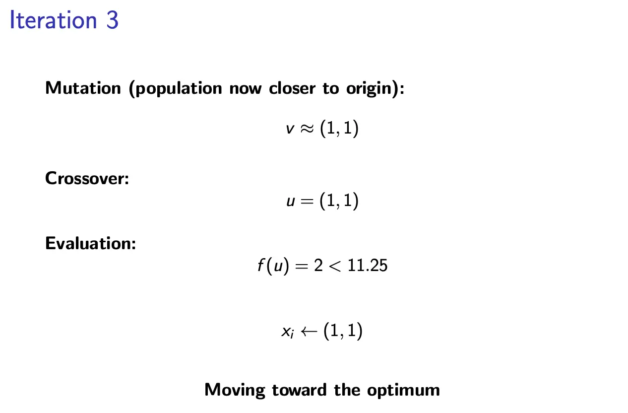
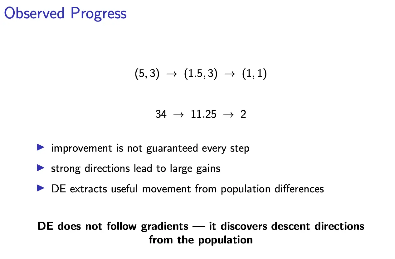
Examples
Small Numerical Example
Full DE Step Example