Restricted Boltzmann Machines

An RBM network consists of:

• A “hidden layer”: $\vec{h}\in \{0,1{\}}^n$
• A “visible layer”: $\vec{v}\in \{0,1{\}}^m$, because this layer interacts with the environment.

Note that each node is binary, so it is either on (1) or off (0). The probability that a node is on depends on the states of the nodes feeding it, and the connection weights.

Connections between layers are symmetric, represented by weight matrix $W$.

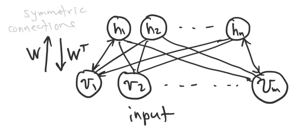
Together, $\vec{v}$ and $\vec{h}$ represent the network state. For example, a single network state could be:

$$\begin{array}{rl}\vec{v}& =\left[\begin{array}{cccc}1& 0& 0& 1\end{array}\right]\\ \vec{h}& =\left[\begin{array}{ccc}0& 1& 1\end{array}\right]\end{array}$$

RBM energy

Similar Hopfield Networks, an RBM is characterized by an energy:

$$\begin{array}{rl}E(v,h)& =-\sum _{i=1}^m\sum _{j=1}^n{v}_i{W}_{ij}{h}_j+\sum _{i=1}^m{b}_i{v}_i+\sum _{j=1}^n{c}_j{h}_j\\ & =-vW{h}^T-v{b}^T-h{c}^T\end{array}$$

• $b$ is a bias for the visible units, $c$ is a bias for the hidden units
• $-vW{h}^T$ is a discount for when nodes $i$ and $j$ are both on
• $-b{v}^T-c{h}^T$ is the energy incurred by turning a node on.

Like many processes in nature, we want to find the minimum energy.

Consider the “energy gap”, the difference in energy when we flip an energy $v_k$ from off to on.

$$\begin{array}{rl}\Delta E_k& =E(v_k\text{ off})-E(v_k\text{ on})\\ & =\sum _j{w}_{kj}{h}_j-b_j\end{array}$$

• If $\Delta E_k>0$, $E(v_k\text{ off})>E(v_k\text{ on})$. Then “on” is lower energy, so we set $v_k=1$
• If $\Delta E_k<0$, $E(v_k\text{ off})<E(v_k\text{ on})$, then “off” is lower energy, so we set $v_k=0$.

The energy gap of each node depends on the states of other nodes, so finding the minimum energy state requires some work. One strategy is to visit and update the nodes in random order (like Hopfield). We can do better since our network is bipartite (hence the “Restricted”). The visible units only depend on the hidden units, and vice versa, so we can update one whole layer at a time.

This is still a local optimization method, so we can still get stuck in local optima. To avoid this, we use stochastic (random) neurons. Each neuron is on or off according to a probability that is established by its input current:

$$\begin{array}{r}P(v_k=1|\vec{h})=\sigma (\Delta E_k)\\ P(h_j=1|\vec{v})=\sigma (\Delta E_j)\\ \sigma (z)=\frac{1}{1+e^{-\frac{z}{T}}}\end{array}$$

where $T$ is a temperature parameter. This idea comes from statistical mechanics. Essentially, higher temperature makes the sigmoid curve flatten so that there is more movement back and fourth between the states.

Let’s say we want to find out whether neuron $h_j\sim P(h_j=1|v)$ is on:

1. Evaluate its input $H=\sigma (\dots )$
2. For $j=1,\dots ,n$:
   • $r=\text{rand}\in (0,1)$
   • If $H_j>r$:
     • $h_j=1$
   • Else:
     • $h_j=0$

This produces a $\vec{h}\in \{(0,1){\}}^n$.

This is basically a Bernoulli Distribution sampling process.

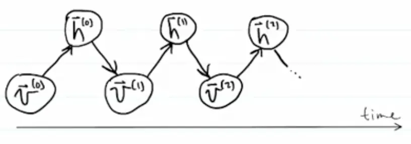
If we let our network run freely using the logistic function to compute the probability that the neuron is 1 vs. 0. Starting with some initial state $v^{(0)}$, we project up to $h^{(0)}$, project it down to get to $v^{(1)}$, project back up, etc…

We will eventually visit all possible network states, but not with equal probability. Instead we will visit state $(\vec{v},\vec{h})$ with probability

$$P(v,h)=\frac{1}{z}{e}^{-E(v,h)}$$

where $z={\sum }_{v,h}{e}^{-E(v,h)}$. This is essentially just softmax.

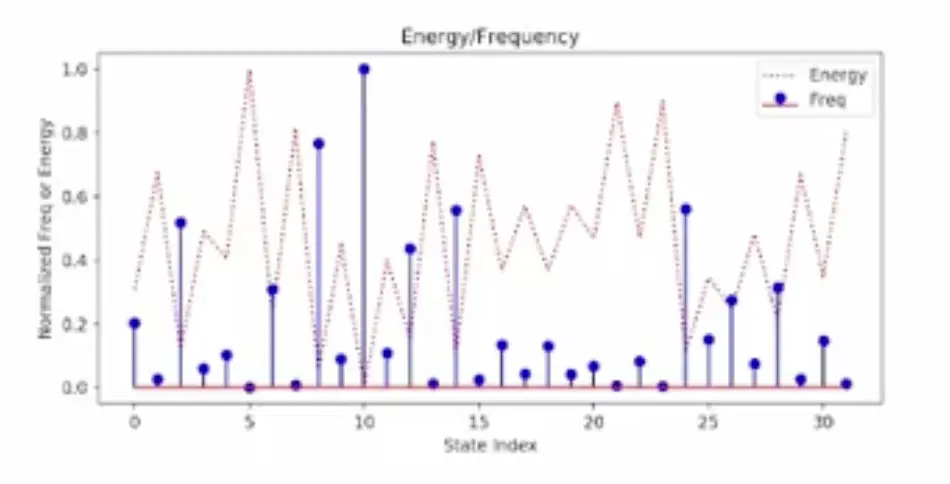
If $E(v^{(1)},h^{(1)})>E(v^{(1)},h^{(1)})$, then the $P(v^{(1)},h^{(1)})<P(v^{(2)},h^{(2)})$. Lower energy states are visited more frequently. This is known as the Boltzmann Distribution.

Example with 4 visible nodes and 2 hidden nodes (32 net states):

Training an RBM as a Generative Model

Suppose we have inputs $v\sim p(v)$. We want an RBM to behave as a generative model $q_{\theta }$ such that:

$$\underset{\theta }{\max }{E}_{v\sim p}[q_{\theta }(v)]\text{or equivalently}\underset{\theta }{\min }{E}_{v\sim p}[-\ln q_{\theta }(v)]$$

Let $L=-\ln q_{\theta }(\vec{\nu })$ for a given fixed $\vec{\nu }$. Then:

$$\begin{array}{rl}L& =-\ln \left(\frac{1}{Z}\sum _h{e}^{-E_{\theta }(\nu ,h)}\right)\\ & =-\ln \left(\sum _h{e}^{-E_{\theta }(\nu ,h)}\right)+\ln \left(\sum _v\sum _h{e}^{-E_{\theta }(\nu ,h)}\right)\\ & =L_1+L_2\end{array}$$

Thus, we can decompose the loss into $L=L_1+L_2$.

To do gradient descent, we need to find the gradients.

Gradient of $L_1$

$${\nabla }_{\theta }{L}_1={\mathbb{E}}_{q(h|\nu )}[{\nabla }_{\theta }{E}_{\theta }]$$

• $q(h|\nu )$ is the distribution of $h$ conditioned on the fixed $\nu$

Gradient of $L_2$

$${\nabla }_{\theta }{L}_2={\mathbb{E}}_{q(v,h)}[-{\nabla }_{\theta }{E}_{\theta }]$$

• $q(v,h)$ is the joint distribution over $v$ and $h$

Gradient for $W_{ij}$

What is the gradient of ${\nabla }_{\theta }{E}_{\theta }$? Consider $\theta =w_{ij}$.

Recall:

$$E(v,h)=-\sum _{i=1}^m\sum _{j=1}^n{v}_i{W}_{ij}{h}_j+\sum _{i=1}^m{b}_i{v}_i+\sum _{j=1}^n{c}_j{h}_j$$

Then:

$$\begin{array}{r}{\nabla }_{w_{ij}}E(\nu ,h)=-{\nu }_i{h}_j\text{and}{\nabla }_{w_{ij}}E(v,h)=-v_i{h}_j\\ \therefore {\nabla }_{w_{ij}}L=\underset{\text{term 1}}{\underbrace{{\mathbb{E}}_{q(h|\nu )}[{\nu }_i{h}_j]}}-\underset{\text{term 2}}{\underbrace{{\mathbb{E}}_{q(v,h)}[v_i{h}_j]}}\end{array}$$

Term 1. This is the expected value under the posterior distribution. We clamp visible states to $\nu$:

$$q(h_i|\vec{\nu })=\sigma (-\vec{\nu }{W}_{ij}+c_j)$$

Note that this calculates the hidden $h_j$ Bernoulli probabilities! It does not actually give us the binary hidden units.

Then

$${\mathbb{E}}_{q(\vec{h}|\vec{\nu })}[{\nu }_i{h}_j]=-{\nu }_i\sigma (-\nu W_{ij}+c_j)$$

Computing for all the weights at once:

$${\nabla }_w{L}_1=-{\vec{\nu }}^T\sigma (-\vec{\nu }W+\vec{c})$$

Term 2. This is the expected value under the joint distribution. Compute:

$${\mathbb{E}}_{q(\vec{v},\vec{h})}[v_i{h}_j]=\sum _{\vec{v}}\sum _{\vec{h}}q(\vec{v},\vec{h})v_i{h}_j$$

We could find this by running the network freely for a lot of iterations and sampling the results. In practice, a single net state is used.

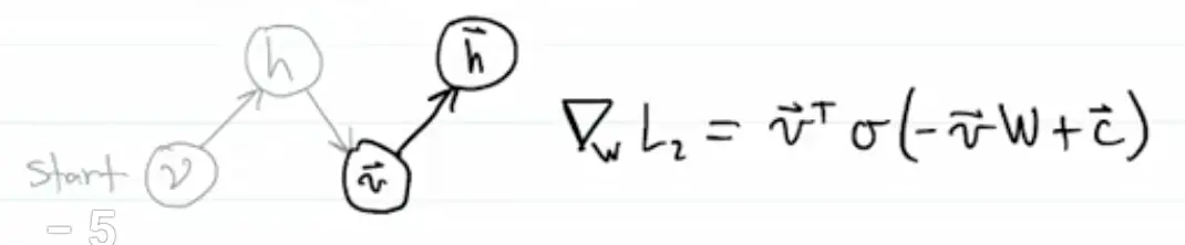
We start with the fixed $\nu$ and then project it up to get the hidden probabilities. This is done as part of the calculation for ${\nabla }_w{L}_1$. Then, we use the probabilities, sample to get a binary $h$. We project down to get a new visible state, and then project up again. We use this $v$ and $h$ as a single sample to get

$${\nabla }_w{L}_2={\vec{v}}^T\sigma (-\vec{v}W+\vec{c})$$

To update all weights in $W$:

$$\begin{array}{rl}W& =W-\kappa ({\nabla }_w{L}_1+{\nabla }_w{L}_2)\\ & =W+\kappa \underset{\text{clamped}}{\underbrace{{\vec{\nu }}^T\sigma (-\vec{\nu }W+\vec{c})}}-\kappa \underset{\text{free}}{\underbrace{{\vec{v}}^T\sigma (-\vec{v}W+\vec{c})}}\end{array}$$

We call the up pass (from visible to hidden) recognition. We call the down pass (hidden to visible) generation.

Contrastive Divergence for Training RBMs

This algorithm is based on a comparison between the original input, and how well it can be reconstructed from the resulting hidden-layer state.

We are given an input pattern $\vec{\nu }$ with $m$ visible nodes and $n$ hidden nodes.

1. Recognition pass 1. Given a visible pattern $\vec{\nu }$, we compute hidden probabilities.

$$P(\vec{h}|\vec{\nu })=\sigma (\overrightarrow{\Delta E})$$

where $\overrightarrow{\Delta E}=-\vec{\nu }W+\vec{c}$.

2. Compute term 1 (the co-occurence statistics): how many times $h$ and $v$ are both on simultaneously>

$$s_1={\vec{\nu }}^T\sigma (\overrightarrow{\Delta E})$$

3. Generative pass: We sample the Bernoulli process for the hidden nodes:

$${\vec{h}}_1\sim \sigma (\overrightarrow{\Delta E})\in \{0,1{\}}^n$$

Projecting down gives us the energy gap for the visible nodes:

$$\overrightarrow{\Delta E}=-W{\vec{h}}_1^T+\vec{b}$$

Computing the Bernoulli probabilities of the visibles given the hidden:

$$P(\vec{\nu }|{\vec{h}}_1)=\sigma (\overrightarrow{\Delta E})$$

Sample ${\vec{v}}_2\sim P(\vec{\nu }|{\vec{h}}_1)\in \{0,1{\}}^m$.

4. Recognition pass 2:

$$\begin{array}{r}\overrightarrow{\Delta E}=-{\vec{v}}_{2}W+\vec{c}\end{array}$$

We can sample ${\vec{h}}_2\sim \sigma (\overrightarrow{\Delta E})$ or use $\sigma (\overrightarrow{\Delta E})$ directly.

5. Compute term 2 co-occurence states:

$$s_2={\vec{v}}_2{h}_2$$

6. Update weights:

$$W_{\text{new}}=W_{\text{old}}+\kappa (s_1-s_2)$$

This is essentially using a reconstruction loss between the co-occurrence statistics for the input ($s_1$) and the co-occurrence statistics for the reconstruction ($s_2$).

Update biases:

$${\vec{b}}_{\text{new}}={\vec{b}}_{\text{old}}-\gamma (\vec{\nu }-{\vec{v}}_2)$$ $${\vec{c}}_{\text{new}}={\vec{c}}_{\text{old}}-\gamma ({\vec{h}}_1-{\vec{h}}_2)$$

Training algorithm:

for each temp T = 20, 10, 5, 2,1
    for each of 400 epochs
        for each V batch (visibles from data)
            add some noise (optional)
            project up: V -> H1, collect S1
            project down & up: H1 -> V1 -> H2: Collect S2
            update weights & biases

1. Look at the real data and infer which hidden features are probably present.
2. Record the visible-hidden associations found in the real data.
3. Sample hidden features and use them to reconstruct the visible pattern.
4. Look at the reconstruction and infer which hidden features it implies.
5. Record the visible-hidden associations found in the reconstruction.
6. Adjust parameters so real-data associations become more likely and reconstruction-only associations become less likely.