Contours in Complex Plane

Consider a simple closed-loop curve $\Gamma$, which segments the complex plane into a region that is inside the curve and a region that is outside the curve.

[Figure]

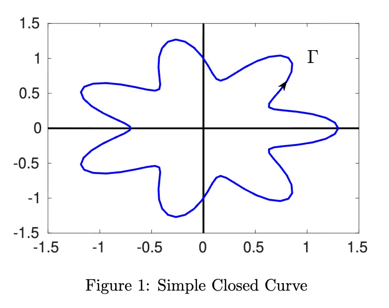
Some terminology

• Simple: No self-intersections
• Closed: Curve starts and ends at the same point (i.e., no end points)

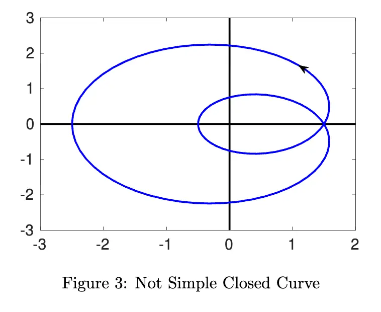
Note that the curves have directionality; an arrow tells us which way to travel around the curve.

Definition: Contour

$\Gamma$ is a contour if it is a simple closed curve with a direction.

Contour Integration

Let’s do a contour integration example with a unit circle. First, we define a contour $\Gamma$ that is a circle centered at $\rho \in \mathbb{C}$ with radius $r>0$:

$$\Gamma =\{\rho +r{e}^{j\theta }:\theta \in [0,2\pi ]\}$$

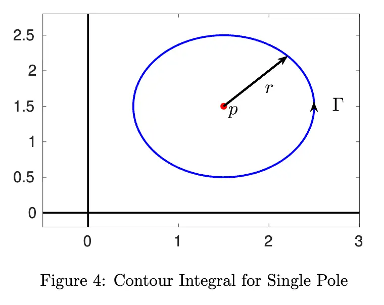
Now, let’s compute the integral, assuming the pole $p$ is at the center of the circle (i.e. $p=\rho$):

$$\frac{1}{2\pi j}{\oint }_{\Gamma }\frac{1}{z-p}dz$$

We do a change of coordinates:

$$\begin{array}{rl}z& =p+r{e}^{j\theta }\\ dz& =jr{e}^{j\theta }d\theta \end{array}$$

Substitute into the integral:

$$\begin{array}{rl}\frac{1}{2\pi j}{\oint }_{\Gamma }\frac{1}{z-p}dz& =\frac{1}{2\pi j}{\int }_0^{2\pi }\frac{1}{(p+r{e}^{j\theta }-p)}\cdot (jr{e}^{j\theta }d\theta )\\ & =\frac{1}{2\pi j}{\int }_0^{2\pi }\frac{1}{r{e}^{j\theta }}\cdot (jr{e}^{j\theta }d\theta )\\ & =\frac{1}{2\pi j}{\int }_0^{2\pi }jd\theta \\ & =\frac{1}{2\pi j}[j\theta {]}_0^{2\pi }=\frac{j2\pi }{2\pi j}=1\end{array}$$

When we integrated along a circular contour centered on a pole $p$, we got an answer of $1$. This is not a coincidence; more generally, we have the following rule:

Lemma 1 (Cauchy's Integral Formula - special case)

Let $p\in \mathbb{C}$. Let $\Gamma$ be a contour. Then,

$$\frac{1}{2\pi j}{\oint }_{\Gamma }\frac{1}{z-p}dz=\{\begin{array}{ll}1,& \text{if }\Gamma \text{ encloses }p\\ 0,& \text{otherwise}\end{array}$$

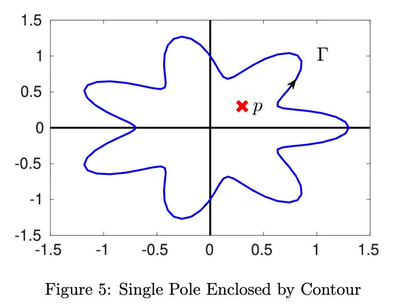
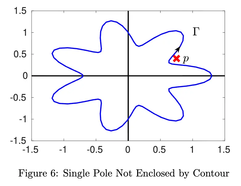
So as long as $p$ is inside of $\Gamma$, the integral will always evaluate to $1$. It doesn’t depend on $\Gamma$ being a circle – $\Gamma$ can take any shape and this will still hold true.

This will basically let us count up how many poles are inside and how many poles are outside the unit disk.

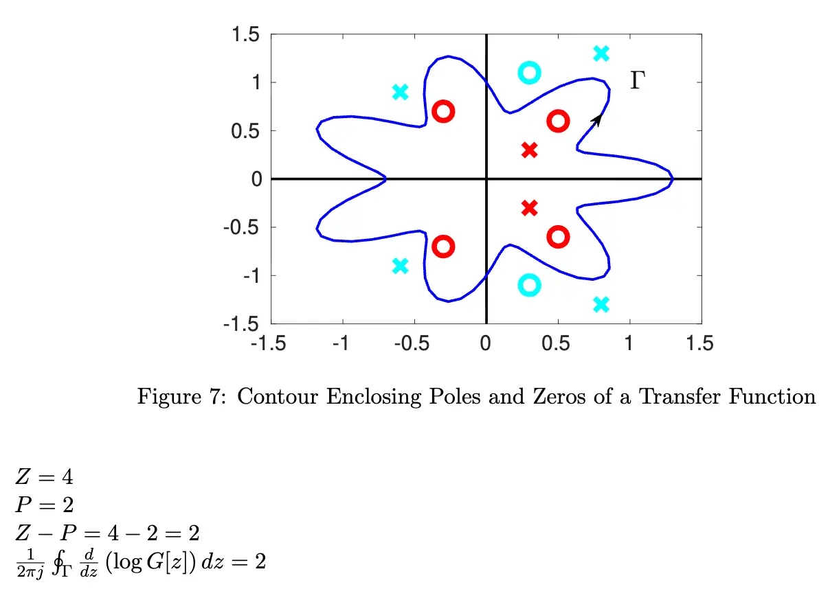
Connecting to Transfer Functions

Let $G[z]$ be real, rational, and proper. Let $\Gamma$ be a contour. Then, $G[z]$ can be written as:

$$G[z]=k\cdot \frac{{\prod }_{j=1}^m(z-z_j)}{{\prod }_{i=1}^n(z-p_i)}$$

where $z_j,p_i$ are the zeros and poles of $G[z]$ respectively. Our goal is to simplify this expression to take it toward the form of $\frac{1}{z-p}$.

First, we take the log:

$$\log (G[z])=\log (k)+\sum _{j=1}^m\log (z-z_j)-\sum _{i=1}^n\log (z-p_i)$$

Differentiating with respect to $z$:

$$\frac{d}{dz}(\log (G[z]))=\sum _{i=1}^m\frac{1}{z-z_j}-\sum _{i=1}^n\frac{1}{z-p_i}$$

Now integrating this over the contour $\Gamma$ and multiplying by $\frac{1}{2\pi j}$:

$$\begin{array}{rl}\frac{1}{2\pi j}{\oint }_{\Gamma }\left(\frac{d}{dz}\log (G[z])\right)dz& =\frac{1}{2\pi j}{\oint }_{\Gamma }\left(\sum _{j=1}^m\frac{1}{z-z_j}-\sum _{i=1}^n\frac{1}{z-p_i}\right)dz\\ & =\sum _{j=1}^m\left[\frac{1}{2\pi j}{\oint }_{\Gamma }\frac{1}{z-z_j}dz\right]-\sum _{i=1}^n\left[\frac{1}{2\pi j}{\oint }_{\Gamma }\frac{1}{z-p_i}dz\right]\end{array}$$

Applying our lemma:

$$\begin{array}{rl}\text{Integral}& =\sum _{j=1}^m\{\begin{array}{ll}1,& \text{if }\Gamma \text{ encloses }{z}_j\\ 0,& \text{otherwise}\end{array}-\sum _{i=1}^n\{\begin{array}{ll}1,& \text{if }\Gamma \text{ encloses }{p}_i\\ 0,& \text{otherwise}\end{array}\\ & =Z-P\end{array}$$

Therefore, we can evaluate this integral by just looking at $\Gamma$ and the poles/zeros of $G[z]$, but this doesn’t help us that much yet. This way tells us about the the relationships between the number of poles and the number of zeros. But we can calculate it in a different way.

We can evaluate the integral in a different way using a change of variables:

$$\frac{1}{2\pi j}{\oint }_{\Gamma }\left(\frac{d}{dz}\log (G[z])\right)dz=\frac{1}{2\pi j}{\oint }_{\Gamma }\frac{G^{\prime }[z]}{G[z]}dz$$

• via the chain rule, where $G^{\prime }[z]=\frac{dG}{dz}$

Consider a new variable:

$$\begin{array}{rl}w& =G[z]\\ dw& =G^{\prime }[z]dz\end{array}$$

Substituting this into the integral, we change the integration path from $\Gamma$ to $G[\Gamma ]$:

$$\frac{1}{2\pi j}{\oint }_{\Gamma }\frac{G^{\prime }[z]}{G[z]}dz=\frac{1}{2\pi j}{\oint }_{G[\Gamma ]}\frac{dw}{w}$$

This new integral represents the number of times the mapped contour $G[\Gamma ]$ encircles the origin.

To explain what $G[\Gamma ]$ is, we did a change of variables, so we have to do a change over what we are integrating over. $G[\Gamma ]$ takes every point on $\Gamma$, and maps it with the function $G$. In general, $G[\Gamma ]$ is closed but not simple.

Let $w=G[z]$ so the integral becomes $\frac{1}{2\pi j}{\oint }_{G[\Gamma ]}\frac{dw}{w}$.

We represent $w$ in polar coordinates $w=r{e}^{j\theta }$. The differential $dw$ is:

$$dw=\frac{\partial w}{\partial r}dr+\frac{\partial w}{\partial \theta }d\theta =e^{j\theta }dr+jr{e}^{j\theta }d\theta$$

Therefore, $\frac{dw}{w}$ simplifies nicely:

$$\frac{dw}{w}=\frac{e^{j\theta }dr+jr{e}^{j\theta }d\theta }{r{e}^{j\theta }}=\frac{dr}{r}+jd\theta$$

Now, we can evaluate our integral:

$$\begin{array}{rl}\frac{1}{2\pi j}{\oint }_{G[\Gamma ]}\frac{dw}{w}& =\frac{1}{2\pi j}{\oint }_{G[\Gamma ]}\left(\frac{dr}{r}+jd\theta \right)\\ & =\frac{1}{2\pi j}[\log (r)+j\theta {]}_{\text{start}}^{\text{end}}\\ & =\frac{1}{2\pi j}[(\log (r_1)-\log (r_0))+j({\theta }_1-{\theta }_0)]\end{array}$$

Since $G[\Gamma ]$ is a closed curve, the start and end points $(r_0,{\theta }_0)$ and $(r_1,{\theta }_1)$ must have the same magnitude, so $r_1=r_0$. This means the $\log (r)$ term goes to zero:

$$\begin{array}{rl}& =\frac{1}{2\pi j}[0+j({\theta }_1-{\theta }_0)]\\ & =\frac{j(\Delta \theta )}{2\pi j}=\frac{\Delta \theta }{2\pi }\end{array}$$

The total change in angle, $\Delta \theta$, must be an integer multiple of $2\pi$ for a closed loop. We can write $\Delta \theta =2\pi N$, where $N$ is this integer:

$$\frac{2\pi N}{2\pi }=N$$

Therefore, this integral simply counts $N$, the number of times the mapped contour $G[\Gamma ]$ encircles the origin.