Simple Generator

See:

• EMF Generation with Conductor Relative Motion
• Generation of Force with Conductor in a Magnetic Field

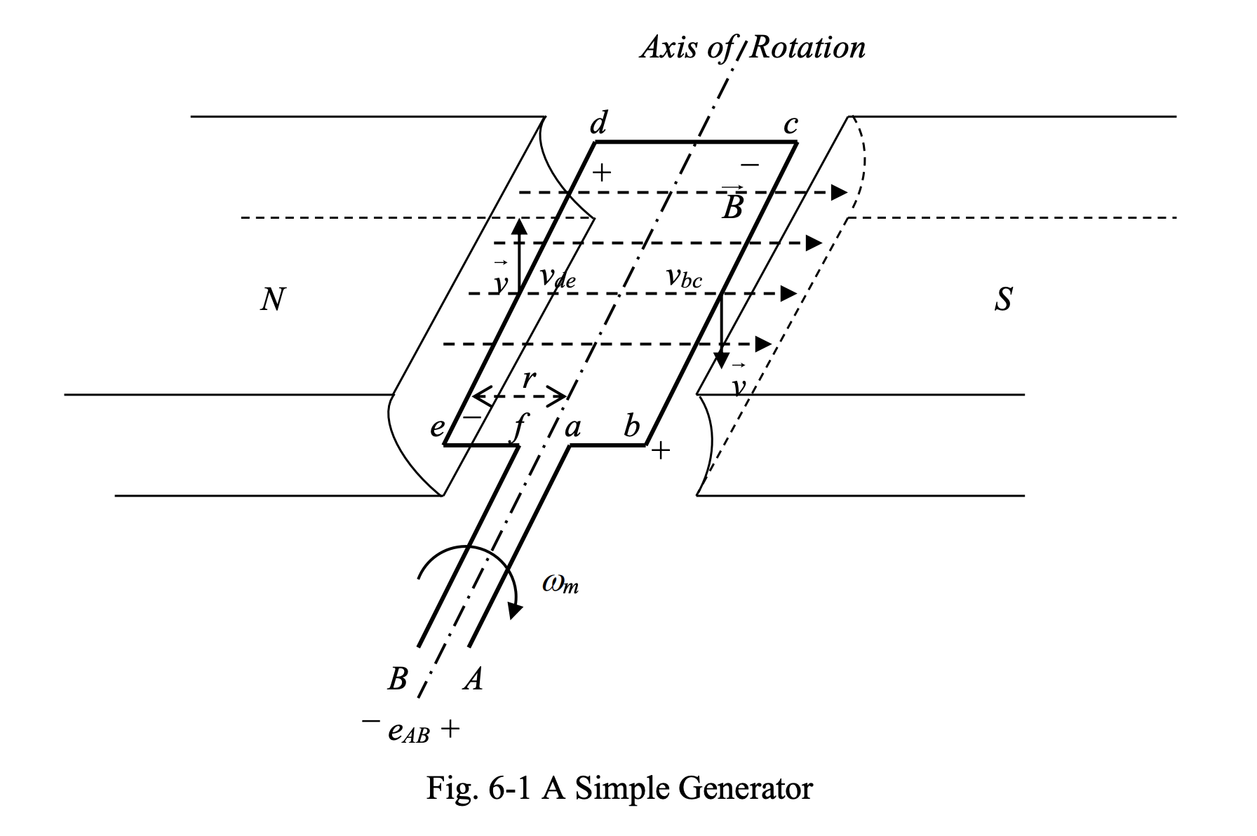
To explain the structure and operation of DC machines, let’s consider a loop of wire rotating about its axis in a constant uniform magnetic field produced by a permanent magnet, as shown in Fig. 6-1.

In any arbitrary position of the loop, the emf is induced in different segments of the loop of wire can be found by:

$$\begin{array}{r}{\vec{e}}_{\text{induced}}=(\vec{v}\times \vec{B})\cdot \vec{l}\end{array}$$

where $\vec{v},\vec{B},\vec{l}$ are the vectors of linear speed, magnetic flux density and length of conductor. Note that the magnitude of $\vec{l}$ is equal to the length of the conductor and its direction is such that it makes an angle between $0°$ and $90°$ with $\vec{v}\times \vec{B}$ . If $\vec{v}\times \vec{B}$ is collinear with $\vec{l}$ , $(1)$ simplifies to:

$${\vec{e}}_{\text{induced}}=(\vec{v}l\times \vec{B})$$

Also, if $\vec{v}\perp \vec{B}$ , $|\vec{v}\times \vec{B}|=vB\sin 90°=vB$, and $|{\vec{e}}_{\text{induced}}|=vBl$. This is the largest emf that can be induced in a conductor of length $l$, when moving at the velocity of $v$ in a magnetic field of magnetic flux density $B$.

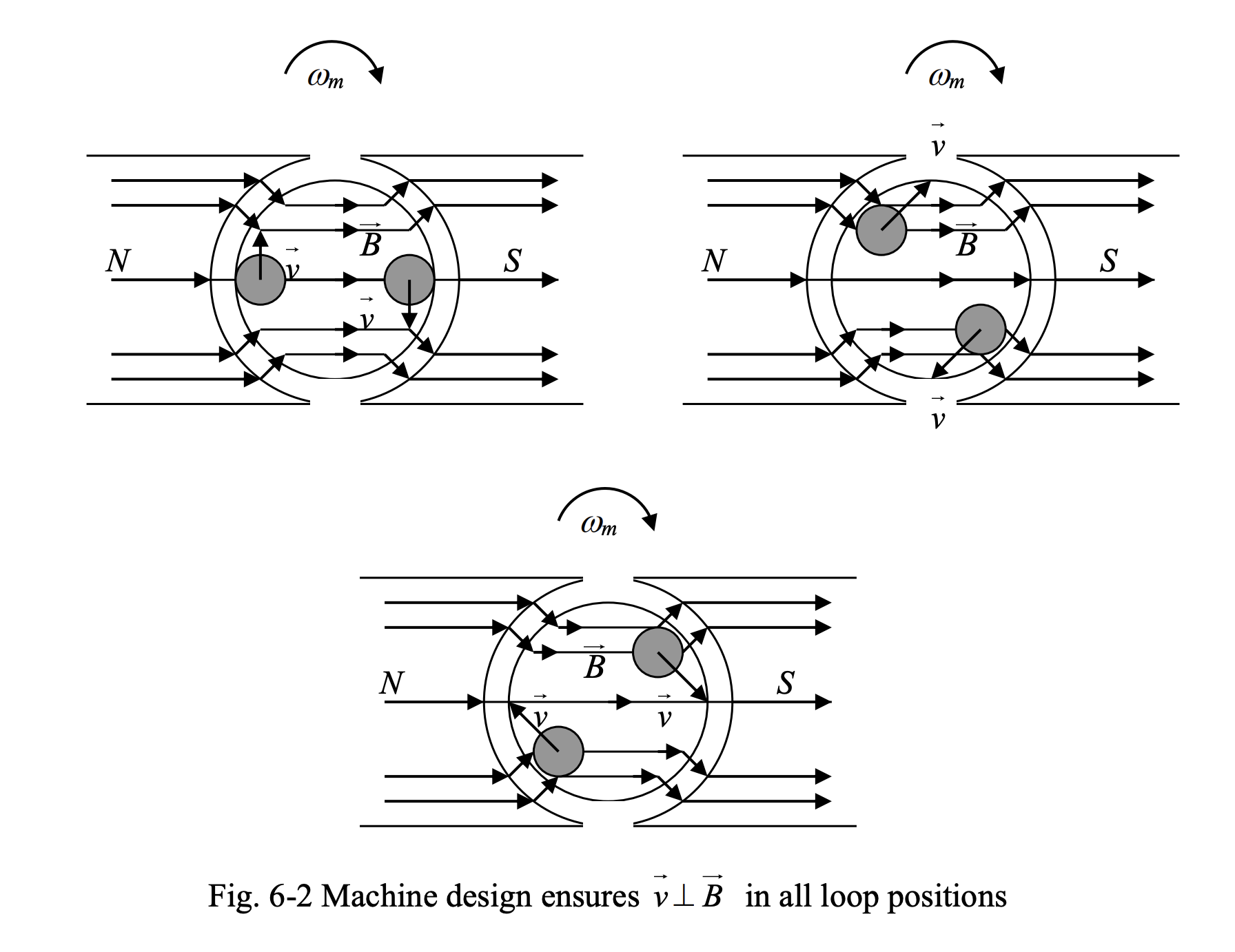
The practical electric machines are designed such that $v\perp B$ at almost all possible positions of the loop. This is accomplished by giving the pole faces a circular shape, as shown in Fig. 6-2, and reducing the time period during which the loop is not under the pole faces to a minimum. Also, we try to make $\vec{v}\times \vec{B}$ collinear with $l$ for the segments of the loop participating in voltage generation. This ensures the best utilization of the installed capacity of the machine.

Segment EMFs

We can find the induced emfs in different segments of the loop shown in Fig. 6-1.

• ab, ef, cd: For these conductor segments, $(\vec{v}\times \vec{B})\times \vec{l}$. thus $e_{\text{induced}}=0$.
• bc: For conductor segment bc, $\vec{v}\perp \vec{B}$ and $\vec{v}\times \vec{B}$ is collinear with $l$. Therefore, as long as the loop side bc is under the S pole face, we have:

$$e_{\text{induced},bc}=vB{l}_{bc}$$

• de: For conductor segment de, $v\perp B$ and $\vec{v}\times \vec{B}$ is collinear with $l$. Therefore, as in the case of segment bc, as long as the loop side de is under the N pole face, we have:

$$e_{\text{induced},de}=vB{l}_{de}$$

As a result, the total emf in the loop will be:

$$e_{AB}=e_{\text{induced},ab}+e_{\text{induced},bc}+e_{\text{induced},cd}+e_{\text{induced},de}+e_{\text{induced},ef}$$

If $l_{bc}=l_{de}=l$, then:

$$e_{AB}=2vBl$$

The voltage $e_{AB}$ given corresponds to the loop position illustrated in Fig 6-1.

As the loop rotates, for half a revolution, or $180°$:

• bc is under the face of the south pole
• de is under the face of the north pole,
• $e_{AB}=2vBl$.

Thus, it can be concluded that the output voltage will have a constant value of $2vBl$ for as long as the situation is as described above.

When the loop sides leave the pole faces, $v$ and $B$ make an angle of $0°$ and $180°$, and thus, $\vec{v}\times \vec{B}=0$ . Therefore, beyond pole faces, we have:

$$\begin{array}{rl}{e}_{AB}& =e_{\text{induced},ab}+e_{\text{induced},bc}+e_{\text{induced},cd}+e_{\text{induced},de}+e_{\text{induced},ef}\\ & =0+0+0+0+0=0\end{array}$$

During the next half revolution or $180°$, when the loop side bc will be under the face of the north pole and the loop side de under the face of the south pole, as shown in Fig. 6-3.

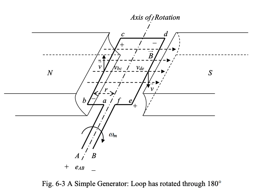
The emfs induced in the loop sides bc and de will change polarity, while keeping the same magnitude. This is because the angle between $\vec{v}$ and $\vec{B}$ changes sign from $90°$ to $-90°$. For ab, cd and ef segments, we again have $(\vec{v}\times \vec{B})\perp \vec{l}$, and thus, $e_{\text{induced}}=0$. Therefore, during the second half of a revolution, we have:

$$\begin{array}{rl}{e}_{AB}& =e_{\text{induced},ab}+e_{\text{induced},bc}+e_{\text{induced},cd}+e_{\text{induced},de}+e_{\text{induced},ef}\\ & =0-vB{l}_{bc}+0-vB{l}_{de}+0\\ & =-2vBl\end{array}$$

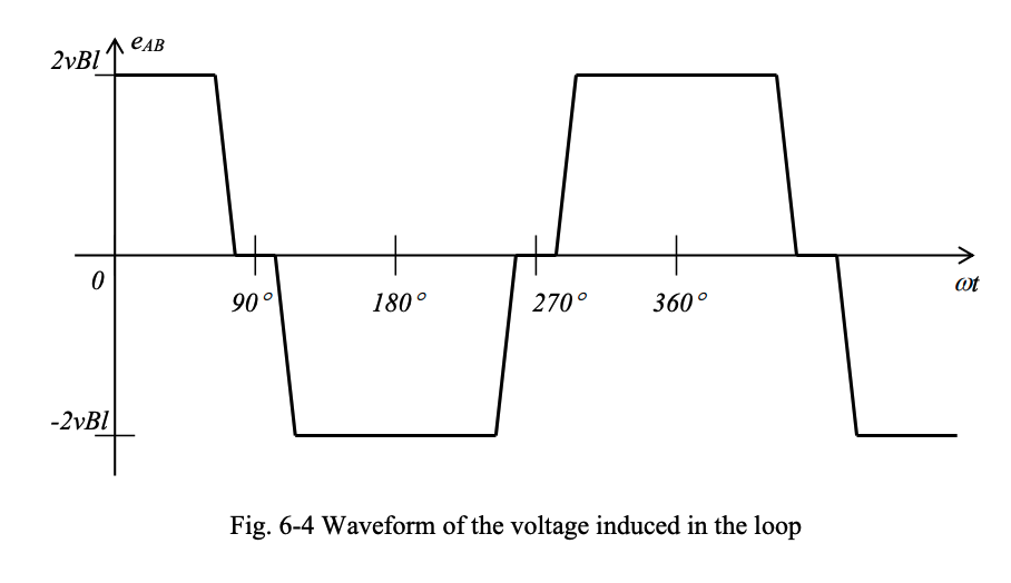
The waveform on the induced emf in the loop will look like that shown below in Fig. 6-4. Note that $e_{AB}$ is either at $2vBl$ or $-2vBl$, with a quick transition between the two levels and a short period at zero, since the loop sides leave the pole faces for only a very short period of time during each revolution.

We can also re-write the above equations by expressing linear speed $v$ in terms of rotational speed, such that:

$$v=r{\omega }_m$$

where $r$ is the radius of the loop and ${\omega }_m$ is the angular speed in radians per second. ${\omega }_m$ can be written as:

$${\omega }_m=\frac{2\pi n}{60}$$

where $n$ is speed in RPM. Therefore,

$$v=r{\omega }_m=r\frac{2\pi n}{60}=\frac{2\pi rn}{60}$$

and

$$e_{AB}=\{\begin{array}{l}2vBl=2\frac{2\pi rn}{60}Bl=\frac{4(\pi rl)Bn}{60}=\frac{4A_{p}Bn}{60}=\frac{4\varphi n}{60}=\frac{\varphi n}{15}\\ \text{or}\\ -2vBl=-\frac{\varphi n}{15}\\ \text{or}\\ 0\end{array}$$

In the above equation, $A_p$ is the area of each pole face, assuming that the length of the air gap between the rotating part (rotor) and stationary part (stator) is negligible compared with other dimensions of the machine. $A_p$ is half of the surface area of a sylinder of radius $r$ and length $l$, or $\frac{1}{2}(2\pi rl)$. We also replaced $A_{p}B$ with $\varphi$.