Spline Interpolation

A spline is a lower order polynomial applied to a subset of points in the data set. A polynomial interpolation fits one curve to all points, while a spline interpolation fits them one curve per interval.

Linear Spline Interpolation

For $n$ data points, there are $i=1$ to $n-1$ intervals. Each interval can be described by a function.

For linear interpolation, each interval can be described by its interval, intercept and slope:

$$\begin{array}{rl}\text{Interval: }& s_i(x)=a_i+b_i(x-x_i),x_i\le x\le x_{i+!}\\ \text{Intercept: }& a_i=f_i\\ \text{Slope: }& b_i=\frac{f_{i+1}-f_i}{x_{i+1}-x_i}\end{array}$$

Combining these, the whole spline would look like:

$$s_i(x)=f_i+\frac{f_{i+1}-f_i}{x_{i+1}-x_i}(x-x_i)$$

Notes

The weakness of linear splines is the abrupt transitions at data points (known as knots). Smooth transitions at knots requires that the function value, and the derivative(s) be equal at each data point. For example, a second‐order spline is continuous in magnitude and
first derivative at the data points.

Quadratic Spline Interpolation

A quadratic spline has the form:

$$s_i(x)=a_i+b_i(x-x_i)+c_i(x-x_i{)}^2$$

For $n$ data points there would be $n-1$ intervals and thus $3(n-1)$ constants $a_i,b_i,c_i$.

At a given interval, $a_i=f_i$, so

$$s_i(x)=f_i+b_i(x-x_i)+c_i(x-x_i{)}^2$$

so our number of constants is reduced to $2(n-1)$ constants $b_i,c_i$.

The functions have to be equal at both knots $i$ and $i+1$, such that

$$\underset{\text{Interval i evaluated at point i+1}}{\underbrace{f_i+b_i(x_{i+1}-x_i)+c_i(x_{i+1}-x_i{)}^2}}=\underset{\text{Interval i+1 evaluated at point i+1}}{\underbrace{f_{i+1}+b_{i+1}(x_{i+1}-x_{i+1})+c_{i+1}(x_{i+1}-x_{i+1}{)}^2}}$$

We can simplify this by letting $h_i=x_{i+1}-x_i$, which allows us to write the above expression as:

$$f_i+b_i{h}_i+c_i{h}_i^2=f_{i+1}$$

This gives us $n-1$ equations (one for each interval from $1\dots n-1$). We still need another $n-1$ equations to solve for coefficients. We find these by enforcing continuity of first derivative (slope) at the interior points. For each interval:

$$s_i^{\prime }(x)=b_i+2c_i(x-x_i)$$

At each point, we check that the slope is continuous by checking

$$b_i+2c_i{h}_i=b_{i+1}$$

where $h_i=x_{i+1}-x_i$.

This gives us $n-2$ more equations, which means we need one more equation. In the absence of additional information, we can assume that the second derivative is zero at the first data point. This is a common approach to generate the last equation, and results in:

$$c_1=0$$

which implies that the first 2 points are connected by a straight line.

At this point, we can form a system of equations for the constants and solve it.

Cubic Spline Interpolation

We determine the coefficients for 3rd order polynomials corresponding to each interval:

$$s_i(x)=f_i+b_i(x-x_i)+c_i(x-x_i{)}^2+d_i(x-x_i{)}^3$$

As before, we enforce:

1. Cubics join at the knots (continuity in magnitude)
2. First derivative of interior knots must be equal (continuity of first derivative)
3. Second derivative of interior knots must be equal (continuity of second derivative)
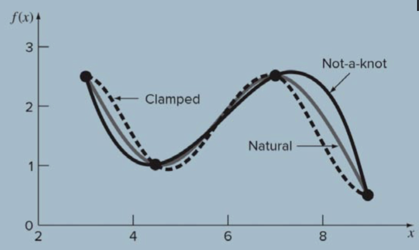
4. To get the required number of equations, we need 2 more conditions. Some options are:
   • Nature spline (second derivatives = 0 at end points)
   • Clamped end condition (first derivatives = 0 at the end points)
   • Not-a-knot end condition (force continuity of the third derivative at the second and next‐to‐last knots)