Finite Element Method - 1D Poisson

Consider the 1D Poisson’s equation:

$$\frac{d^{2}T}{d{x}^2}=-f(x),T(0,t)=T_1,T(L,t)=T_2$$

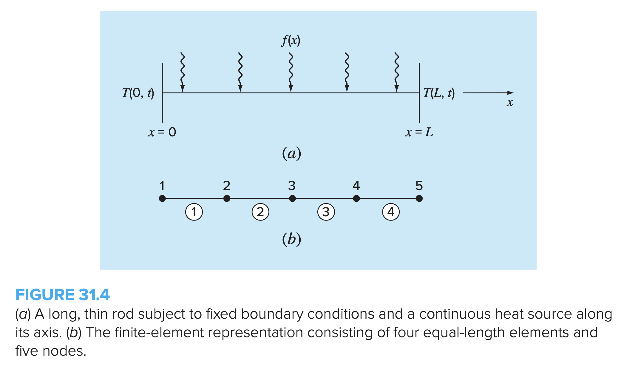
This describes the temperature in a rod with boundary conditions and where $f(x)$ defines a heat source along the length of the rod (10cm).

Analytical Solution

We can solve this by considering the analytical solution form of a quadratic:

$$\begin{array}{r}T=a{x}^2+bx+c\\ T^{\prime \prime }=2a\end{array}$$

The boundary conditions Solving for $a,b,c$ using boundary conditions:

$$\begin{array}{rl}f(x)& =10\\ T^{\prime \prime }& =2a=-f(x)\\ a& =-5\end{array}$$

Boundary conditions:

$$\begin{array}{r}T(0,t)=40\\ T(10,t)=200\end{array}$$

Analytical solution:

$$T=-5x^2+66x+40$$

FEM: Direct Method

If we assume $f(x)=0$, a direct method can be employed to generate the element equations.

The relationship between heat flux and temperature gradient can be represented by Fourier’s Law:

$$q=-k^{\prime }\frac{dT}{dx}$$

where $q=\text{flux}[\text{cal/}({\text{cm}}^2\text{s})]$ and $k^{\prime }$ is the coefficient of thermal conductivity. If a linear approximation function is used to characterize the element’s temperature, the heat flow into the element through node 1 can be represented by:

$$q_1=k^{\prime }\frac{T_1-T_2}{x_2-x_1}$$

where $q_1$ is heat flux at node 1. Similarly, for node 2:

$$q_1=k^{\prime }\frac{T_2-T_1}{x_2-x_1}$$

These two equations express the relationship of the element’s internal temperature distribution (as reflected by the nodal temperatures) to the heat flux at its ends. As such, they constitute our desired element equations.

They can be simplified further by recognizing that Fourier’s law can be used to couch the end fluxes themselves in terms of the temperature gradients at the boundaries:

$$q_1=-k^{\prime }\frac{dT(x_1)}{dx},q_2=k^{\prime }\frac{dT(x_2)}{dx}$$

which can be substituted into the element equations to give

$$\frac{1}{x_2-x_1}\left[\begin{array}{cc}1& -1\\ -1& 1\end{array}\right]\left\{\begin{array}{c}{T}_1\\ T_2\end{array}\right\}=\left\{\begin{array}{c}-\frac{dT(x_1)}{dx}\\ \frac{dT(x_2)}{dx}\end{array}\right\}$$

FEM: Method of Weighted Residuals

This is similar to the direct method but also includes external effects.

The differential equation can be re-expressed as:

$$0=\frac{d^{2}T}{d{x}^2}+f(x)$$

The approximate solution is:

$$\tilde{T}=N_1{T}_1+N_2{T}_2$$

This can be substituted into this equation, which will result in a residual:

$$R=\frac{d^2\tilde{T}}{d{x}^2}+f(x)$$

The method of weighted residuals consists of finding a minimum for the residual according to the general formula

$${\int }_{D}R{W}_{i}dDi=1,2,\dots ,m$$

where $D$ is the solution domain and $W_i$ are linearly independent weighting functions.

We need to decide on weighting functions. One common approach is to use the interpolation functions $N_i$ as the weighting functions (Galerkin’s method), such that:

$${\int }_{D}R{N}_{i}dDi=1,2,\dots ,m$$

For our one-dimensional rod, our previous residual $R=\frac{d^2\tilde{T}}{d{x}^2}+f(x)$ can be substituted into this formulation to give:

$${\int }_{x_1}^{x_2}\left[\frac{d^2\tilde{T}}{d{x}^2}+f(x)\right]N_{i}dxi=1,2$$

which can be re-expressed as:

$${\int }_{x_1}^{x_2}\frac{d^2\tilde{T}}{d{x}^2}{N}_{i}dx=-{\int }_{x_1}^{x_2}f(x)N_i(x)dxi=1,2$$

This solves to:

$$\frac{1}{x_2-x_1}\left[\begin{array}{cc}1& -1\\ -1& 1\end{array}\right]\left\{\begin{array}{c}T\end{array}\right\}=\left\{\begin{array}{c}-\frac{dT(x_1)}{dx}\\ \frac{dT(x_2)}{dx}\end{array}\right\}+\left\{\begin{array}{c}{\int }_{x_1}^{x_2}f(x)N_1(x)dx\\ {\int }_{x_1}^{x_2}f(x)N_2(x)dx\end{array}\right\}$$

So, given our boundary conditions of:

$$\begin{array}{rl}T(0,t)& =40\\ T(10,t)& =200\end{array}$$

Given $f(x)=10$ and elements of length 2.5cm. We have:

• Heat source term, first row:

$${\int }_0^{2.5}10\frac{2.5-x}{2.5}dx=12.5$$

• Heat source term, second row:

$${\int }_0^{2.5}10\frac{x-0}{2.5}dx=12.5$$

For a single element:

$$\begin{array}{rl}0.4T_1-0.4T_2& =-\frac{dT}{dx}(x_1)+12.5\\ -0.4T_1+0.4T_2& =-\frac{dT}{dx}(x_2)+12.5\end{array}$$

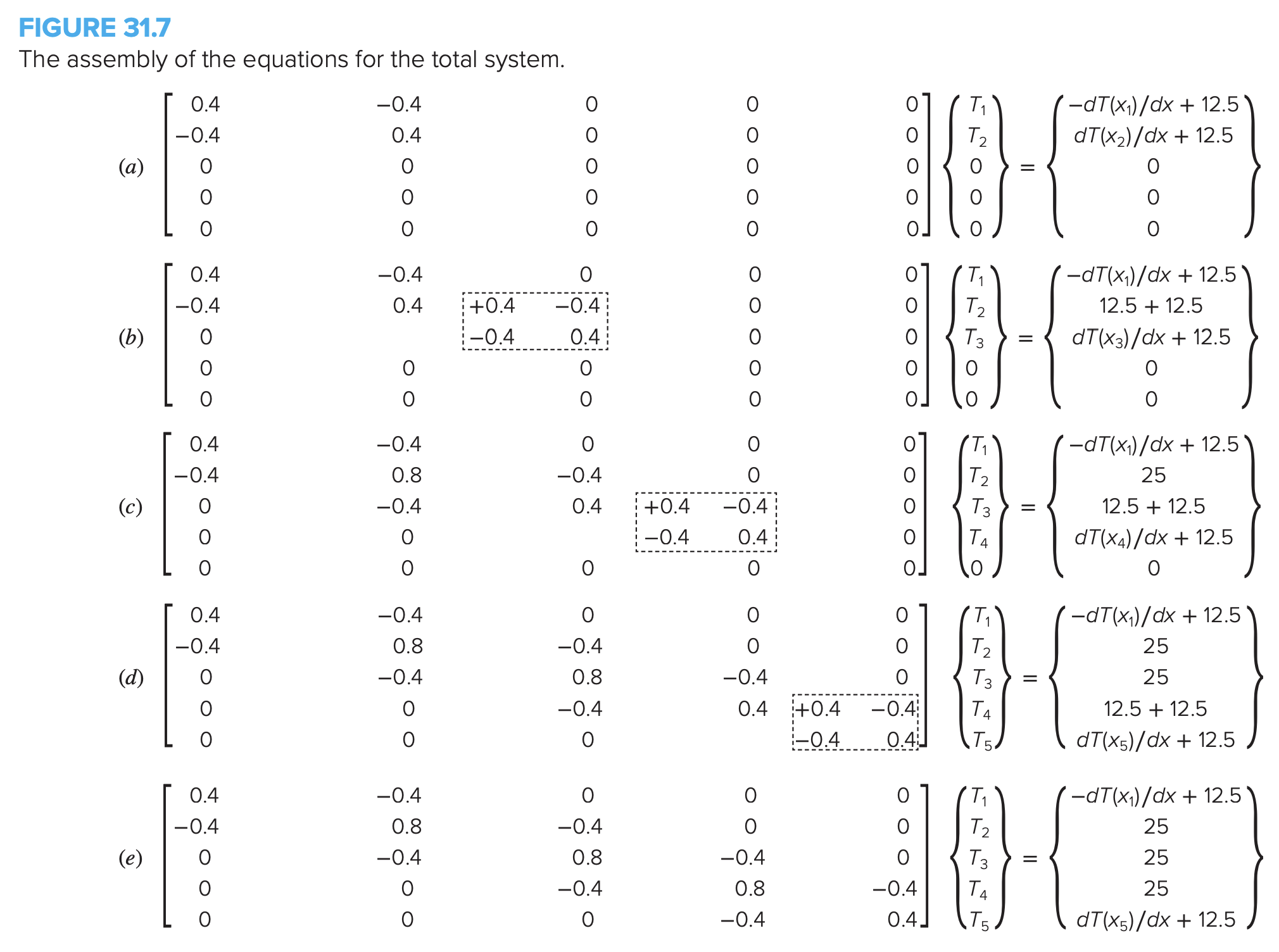
Assembly of equations for the total system:

The boundary conditions are then:

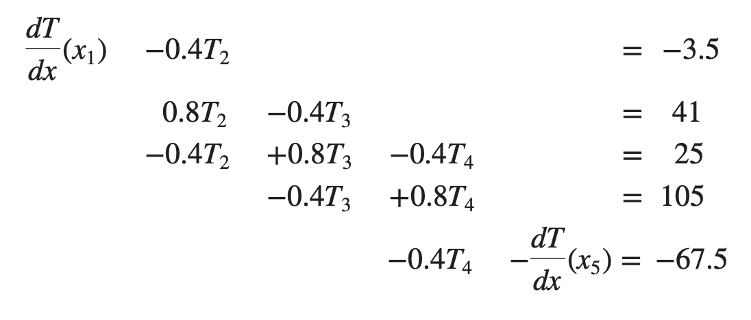
Solution:

$$\begin{array}{rl}\frac{dT}{dx}(x_1)& =66\\ T_2& =173.75\\ T_3& =245\\ T_4& =253.75\\ \frac{dT}{dx}(x_5)& =-34\end{array}$$

Comparison of Analytical vs. FEM

Comparing this analytical solution to our finite element solution:

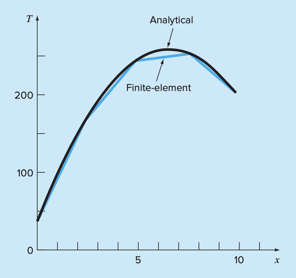
More elements = smoother curve!