Project 2 - Recurrent Neural Networks

Abstract

In the past decade, neural network-based approaches have led to explosive growth in the field of machine learning. Language models are notable and popular application of this with the recent success of GPT \cite{} models. In this report, the mathematical foundations of neural network learning algorithms are examined, with a focus on the backpropagation mechanism. This is slightly extended to introduce the concept of recurrent neural networks and “backpropagation through time”, allowing us to build a basic (but functional) character-level language model. In particular, language model experiments to generate writing in the style of Shakespeare are conducted.

Introduction

Machine learning is often considered an intimidating subject due to its perceived complexity and lack of explanation at high levels, as many complex models appear to be black boxes. However, the foundations of machine learning are relatively simple with a basic understanding of mathematical concepts such as linear algebra and multivariable calculus. Backpropagation is the standard technique for model training as part of the gradient descent process. The objective of this paper is to provide an overview of neural networks and backpropagation, culminating in the introduction of “backpropagation through time” for recurrent neural networks (RNNs). The specific application that is implemented is the generation of text in the style of Shakespeare, which demonstrates the function and capability of RNNs.

In this paper, the following is achieved:

• Using multivariable calculus, we establish the mathematical foundations of feedforward neural networks, which is extended to understand multilayer networks and backpropagation.
• We extend the knowledge of multilayer networks and backpropagation to establish the mathematical foundations of recurrent neural networks and backpropagation through time.
• We implement a recurrent neural network and train it on the writing of William Shakespeare. Model outputs are observed and evaluated, and compared to a more complex 3-layer RNN.

Background

We first introduce the foundational concepts of machine learning by discussing basic feedforward neural networks. This is then extended to recurrent neural networks.

Feedforward Neural Networks

Problem and Data

The core problem in many machine learning tasks is to make accurate predictions or decisions based on input data. In the context of a neural network, this typically involves learning a function that maps input features to desired output labels or values. To achieve this, a model is trained on a dataset comprising numerous instances, each containing a set of features and usually a label or value.

For all of the work discussed in this paper, we are dealing with a supervised learning scenario. This means that the dataset used for training includes not only the input features but also the corresponding output labels, which are essential for the network to learn the correct mappings. This dataset is defined as:

$$D=\{(x^{(1)},y^{(1)}),\dots ,(x^{(n)},y^{(n)})\}$$

where $x$ values indicate inputs features and $y$ values indicate a label of some kind. The specific values and types of $x$ and $y$ dictate the type of problem. For example, sigmoid functions squashes inputs to be between $0$ and $1$, which can be interpreted as probabilities in binary classification tasks. In a multi-layer networks (covered in Sectionref{dafadsf}), this activation and output function may be separated.

Model Definition

At a high-level, neural networks ingest a vector of input features $x=\left[\begin{array}{c}{x}_1,x_2,\dots ,x_n\end{array}\right]$, where $n$ is the number of features. The “features” are individual measurable properties or characteristics of a phenomenon being observed; they inputs that we provide to a model, upon which the model makes a prediction or decision.

The prediction made by the model is fundamentally defined by a set of weights $w=\left[\begin{array}{c}{w}_1,w_2,\dots ,w_n\end{array}\right]$ and a bias term $b$. A weighted sum is produced by taking:

$$z=w^{T}x+b=\sum _{i=1}^n{w}_i{x}_i+b$$

Here, $w^T$ is the transpose of $w$, such that $w^{T}x$ is essentially a dot product. This weighted sum $z$ is called a logit.

At this step, activation functions are usually applied to the weighted logit. Activation functions introduce non-linearity into the network, which allows the network to model more complex relationships between the inputs and outputs. Some examples of activation functions are sigmoid, hyperbolic tangent, and ReLU functions. The activation function can also serves to interpret the output of the network.

We can formalize this entire process as:

$$h(x;w,b)=\sigma (w^{T}x+b)$$

where $h(x;w,b)$ is the hypothesis or the function modeled by the neural network with parameters $w$ (weights) and $b$ (bias), and $\sigma (\cdot )$ represents the activation function applied to the weighted sum of inputs. This is called the forward pass.

Loss Functions

To measure how well the model is performing, a loss function is used. Specifically, loss functions quantify the quality of a prediction $h(x^{(i)};\Theta )$ makes for a specific data sample $(x^{(i)},y^{(i)})$. , where $\Theta$ represents the parameters of the model (such as $w$ and $b$). A low loss value indicates a good prediction, and a high loss indicates a poor prediction.

The exact definition of a loss function depends on the problem at hand. A common loss function for is the binary cross-entropy loss:

$$\begin{array}{r}L(h(x^{(i)};\Theta ),y^{(i)})=\sum _{i=1}^n(y^i\log g^{(i)}+(1-y^{(i)})\log (1-g^{(i)}))\end{array}$$

where $n$ is the number of training examples, $y^{(i)}$ is the true label for the $i^{th}$ training example, and $g^{(i)}$ is the predicted probability output by our model.

Learning as an Optimization Problem

Our model and loss function is defined, but how do we find a model that actually performs well? We can introduce a general framework for training models for arbitrarily complicated problems by framing machine learning as an computational minimization problem.

Fundamentally, we define an objective function $J(\Theta )$, where $\Theta$ are the parameters ($w$ and $b$) of our model. Since the loss function quantifies the quality of our model, we define the objective function to be:

$$J(\Theta )=\left(\frac{1}{n}\sum _{i=1}^n\underset{\text{loss}}{\underbrace{L(h(x^{(i)};\Theta ),y^i)}}\right)$$

such that we are measuring the loss of the model across the entire dataset.

Generally, the optimization is that we want to find ${\Theta }^{\star }$ such that:

$${\Theta }^{\star }={\mathrm{argmin}}_{\Theta }J(\Theta )$$

which is to say that we want to find the $\Theta$ that minimizes $J(\Theta )$, making this a minimization problem.

Training with Gradient Descent

How do we find the minimum of our objective function?

The main idea is if we’re trying to optimize a function f, we compute the gradient at our current point $x$. Since the gradient gives the direction of the maximum rate of increase, we move in the opposite direction, making the function smaller. In terms of a machine learning model, we would have some objective function $J(\Theta )$ defining some surface over $\Theta$, and we want to find the $\Theta$ value at the lowest point on the surface.

We specify an initial value for parameter $\Theta$, a step-size parameter $\eta$ (also called the learning rate), and a convergence threshold $ϵ$. Then, the 1D gradient descent algorithm is:

1. Initialize parameters $\Theta$, learning rate $\eta$, and convergence threshold $\eta$.
2. Repeat until convergence (i.e., when the change in cost function is below $ϵ$):
   1. Compute the gradient ${\nabla }_{\Theta }J(\Theta )$.
   2. Update the parameters: $\Theta \leftarrow \Theta -\eta \cdot {\nabla }_{\Theta }J(\Theta )$.
   3. If the magnitude of the gradient is less than $ϵ$, then stop.
3. Output the final parameters $\Theta$.

\begin{algorithm}
\caption{Gradient Descent} 
\begin{algorithmic}
\State \textbf{Input:} learning rate $\eta$, convergence threshold $\epsilon$
\State \textbf{Output:} optimized parameters $\Theta$
 
\Procedure{GradientDescent}{}
    \State Initialize parameters $\Theta$
    \Repeat
        \State Compute the gradient $\nabla_{\Theta}J(\Theta)$
        \State Update the parameters: $\Theta \leftarrow \Theta - \eta \cdot \nabla_{\Theta}J(\Theta)$
        \If{magnitude of $\nabla_{\Theta}J(\Theta) < \epsilon$}
            \State \textbf{break}
        \EndIf
    \Until{convergence}
    \State \textbf{return} $\Theta$
\EndProcedure
\end{algorithmic}
\end{algorithm}

Multi-layer Neural Networks

Multi-layer networks, often referred to as multi-layer perceptrons (MLPs), extend the concept of the simple neural network model above into a more complex architecture composed of multiple layers of neurons. These layers include:

1. Input Layer: This is the layer that receives the input features. It does not apply any computation and simply passes the features to the next layer.
2. Hidden Layers: One or more layers that compute the intermediate features. These layers are called “hidden” because their outputs are not observed in the training data. The computation in these layers introduces non-linearity to the system, allowing the network to capture complex patterns.
3. Output Layer: The final layer that provides the prediction or classification based on the input features and the computations done by the hidden layers.

The forward pass in multi-layer networks involves sequentially passing the input data passes through each layer to produce an output, such that the output of each layer becomes the input to the next layer. Mathematically, for each layer $l$, this process can be described as:

$$h^{[l]}(x)={\sigma }^{[l]}(w^{[l]T}{h}^{[l-1]}(x)+b^{[l]})$$

where $h^{[l]}(x)$ is the output logit of layer $l$, $w^{[l]}$ and $b^{[l]}$ are the weights and biases of layer $l$, ${\sigma }^{[l]}$ is the activation function for layer $l$, and $h^{[l-1]}(x)$ is the output of the previous layer. We say that $h^{[0]}=x$ is the input to the network and $h^{[L]}$ is the final output (activation of last layer).

The final output layer transforms the outputs of the last hidden layer into a form $y$ that is suitable for the specific type of problem the network is intended to solve. Output layers often use similar functions as activation functions. For example, sigmoid functions squashes inputs to be between $0$ and $1$, which can be interpreted as probabilities in binary classification tasks.

Gradient Descent with Backpropagation

The training process for multi-layer networks follows a similar principle to that of single-layer networks, as discussed in the Training section; we define an objective function and use gradient descent to find model parameters that minimize this objective. The objective function typically includes the loss function $L$ as well as possibly other terms (such as regularization terms). However, the gradient descent process relies on the computation of the gradient of the objective function, $J(\Theta )$. Previously, our $\Theta$ consisted of a single weight and bias, but in a multi-layer network, there are multiple layers of weights and biases; we must find the gradient of the objective function with respect to the weights in the neural network. Backpropagation is a method that uses the chain rule to compute these gradients systematically.

In the introduction of gradient descent in Section, we combined the weights and biases into a single parameter $\Theta =\{w,b\}$. Here, we will consider $w$ and $b$ individually for mathematical clarity.

Let us say we have a multi-layer network with layers $0,\dots ,L$. First, a forward pass is performed. For each layer, we calculate:

$$\begin{array}{rl}{z}^{[l]}& =w^{[l]T}{h}^{[l-1]}+b^{[l]}\\ h^{[l]}& ={\sigma }^{[l]}(z^{[l]})\end{array}$$

where $h^{[0]}=x$ is the input to the network and $h^{[L]}$ is the final output (activation of last layer).

We then compute the loss using the predicted output $h^{[L]}$ and the true value $y$. Then, for the chosen objective function $J(h^{[L]},y)$, we calculate the initial gradient of the loss with respect to the output of the last layer’s activations $\frac{\partial J}{\partial h^{[l]}}$.

Then, we arrive at the central mechanism of backpropagation: the backward pass. This is performed through the network to compute the gradient of the loss with respect to the activations, weights, and biases of each layer, starting from the output layer $L$ back to the first hidden layer.

For the last layer $L$, compute the gradients of the loss with respect to the logits:

$${\delta }^{[L]}=\frac{\partial J}{\partial z^{[L]}}$$

Since $h$ is a function of $z$, we can use the partial derivative chain rule:

$${\delta }^{[L]}=\frac{\partial J}{\partial z^{[L]}}=\frac{\partial J}{\partial h^{[L]}}\cdot \frac{\partial h^{[L]}}{\partial z^{[L]}}$$

where the last term $\frac{\partial h^L}{\partial z^L}$ is the partial derivative of the activation function at the last layer with respect to its input $z^{[L]}$. We use ${\delta }^{[l]}$ to represents the “error” for each layer $l$, quantifying how much a given layer’s output should change to minimize the loss for the entire network.

Then, we compute the gradients for the parameters of each layer. For the output layer $L$, we would have:

$$\begin{array}{rl}{\nabla }_{w^{[L]}}J& ={\delta }^{[L]}\cdot (h^{[L-1]}{)}^T\\ {\nabla }_{b^{[L]}}J& ={\delta }^{[L]}\end{array}$$

Here, the gradient with respect to the bias $b$ is the delta itself because the derivative of $z^{[L]}$ with respect to $b^{[L]}$ is $1$.

Following this method, we can recursive calculate gradients for each preceding layer $l=L-1,L-2,\dots ,1$:

$${\delta }^{[l]}=(w^{[l+1]T}{\delta }^{[l+1]})\cdot \frac{\partial {\sigma }^{[l]}(z^{[l]})}{\partial z^{[l]}}$$

This step propagates the error backward by taking into account the error from the layer above (${\delta }^{[l+1]}$) and the gradient of the activation function for the current layer’s output.

Then, the gradients for the weights and biases for layer $l$ are computed as follows:

$$\begin{array}{rl}{\nabla }_{w^{[l]}}L& ={\delta }^{[l]}\cdot (h^{[l-1]}{)}^T\\ {\nabla }_{b^{[l]}}L& ={\delta }^{[l]}\end{array}$$

Finally, we can update the weights and biases using the previous gradient descent method:

$$\begin{array}{rl}{w}^{[l]}& =w^{[l]}-\eta \cdot {\nabla }_{w^{[l]}}L\\ b^{[l]}& =b^{[l]}-\eta \cdot {\nabla }_{b^{[l]}}L\end{array}$$

Backpropagation is efficient because it calculates the gradients for all weights and biases with only two passes through the network: one forward and one backward. By systematically applying the chain rule, backpropagation avoids redundant computations of gradients, thereby facilitating the training of deep neural networks.

\begin{algorithm} 
\caption{Backpropagation and Gradient Descent} 
\begin{algorithmic}
\Procedure{TrainNetwork}{$D, \eta, \epsilon$}
\STATE Initialize network weights (often small random values) 
\While{not converged} 
\For{each $(x^{(i)}, y^{(i)})$ in training set $D$} 
\State // Forward pass: 
\State Compute activation $a^{[l]}$ for each layer $l$ in the network 
\State // Backward pass: 
\State Compute $\delta^{[L]}$ for output layer $L$ (loss gradient) 
\For{$l = L-1$ to $1$} 
\State Compute $\delta^{[l]}$ based on $\delta^{[l+1]}$ (gradient for layer $l$) 
\EndFor 
\State // Update weights for each layer: 
\For{$l = 1$ to $L$} 
\State Update $w^{[l]} \leftarrow w^{[l]} - \eta \nabla_{w^{[l]}}J(w^{[l]})$ \EndFor 
\EndFor 
\State Check for convergence (e.g., if change in $J(\Theta)$ is below $\epsilon$) 
\EndWhile 
\State 
\Return{network weights} 
\EndProcedure 
\end{algorithmic} 
\end{algorithm}

Recurrent Neural Networks

Based on the background above, we can formulate a recurrent neural network (RNN) in broad terms.

Problem and Data

RNNs are designed to process sequential data, which has many useful applications. For example, when a human reads, we understand each word based on your understanding of previous words. Traditional feedforward neural networks can’t do this; they cannot use its reasoning about previous events in the film to inform later ones.

Reflecting this, the input data for RNNs is usually organized into sequences, and each input example (also known as a sample or instance) is structured as a series of time steps. This means that the input feature $x$ for a single training example is no longer just a vector, but rather a matrix, where each row corresponds to a feature vector at a particular time step. The input to the RNN for each sample is then a matrix $X=[x^{(1)},x^{(2)},\dots ,x^{(T)}]$, where $T$ is the number of time steps.

Similarly, the labels $y$ can also be sequential, representing the desired output at each time step, such that we have $Y=[y^{(1)},y^{(2)},\dots ,y^{(T)}]$.

Model Definition

RNNs are essentially multi-layer networks (see section) in terms of architecture. However, instead of just the output of each layer getting passed to the next, RNNs have a “hidden state” that serves as a form of memory to captures information about what has been processed so far in a sequence. Thus, the output vector’s by the current input and the history of past inputs.

Let us examine the components of RNNs:

1. Input Layer: Similar to MLPs, this layer receives the input features at each time step.
2. Recurrent Layer: One or more layers where each neuron has a recurrent connection to itself, which allows the network to retain the previous state’s information.
3. Output Layer: Produces the prediction for the current time step and can also provide the output for the entire sequence.

The computation of the hidden state at time $t$ can be described as follows:

$$h(t)=\sigma (w_{xh}\cdot x^{(t)}+w_{hh}\cdot h^{(t-1)}+b_h)$$

where:

• $h^{(t)}$ is the hidden state at $t$
• $x^{(t)}$ is the input at time $t$
• $w_{xh}$ are weights connecting the input layer to the hidden layer
• $w_{hh}$ are weights connecting the hidden layer to itself across consecutive time steps. The hidden state from the previous time step $h^{(t-1)}$ is multiplied by these weights.
• $b_h$ is a bias term for hidden state updates.
• $\sigma$ is an activation function for hidden state updates.

The output at time $t$ is then determined by the hidden state, such that:

$$o(t)=\alpha (w_{hy}\cdot h^{(t)}+b_y)$$

where $o(t)$ is the output at time $t$, $w_{hy}$ are weights connecting the hidden state to the output, $b_y$ is an output bias term. We also include an output activation function $\alpha$.

Backpropagation Through Time

Due to the time-dependent nature of RNNs, training them requires an algorithm caleld Backpropagation Through Time (BPTT). BPTT is an extension of the standard backpropagation algorithm, which unfolds the RNN across time steps and then calculates gradients for each time step in the sequence. This allows for the network to be trained on the dependencies across time.

Let us consider an objective function $J(\Theta )$ for RNNs, which typically include the loss computed at each time step, summed over all time steps, such that

$$J(\Theta )=\sum _{t=1}^T{L}^{(t)}(o^{(t)},y^{(t)};\Theta )$$

We’ll denote the objective loss at each timestep $t$ as $J^{(t)}$, which is a function of the true target $y^{(t)}$ and the predicted output $o^{(t)}$.

To update the parameters using gradient descent, we need to calculate the gradient of the objective function with respect to each parameter. For a given parameter $\theta$ in $\Theta$, the gradient is:

$$\frac{\partial J}{\partial \theta }=\sum _{t=1}^T\frac{\partial L^{(t)}}{\partial \theta }$$

Like regular backpropagation, we compute the compute the gradients by applying the chain rule, starting with weights closest to the output and working backwards. For the output weights $w_{hy}$, we note that $J$ is a function of $o^{(t)}$, which is a function of $w_{hy}$. This lets us the gradients are calculated as:

$$\frac{\partial J}{\partial w_{hy}}=\sum _{t=1}^T\frac{\partial L^{(t)}}{\partial o^{(t)}}\frac{\partial o^{(t)}}{\partial w_{hy}}$$

Given $o(t)=\alpha (w_{hy}\cdot h^{(t)}+b_y)$, we have:

$$\frac{\partial o^{(t)}}{\partial w_{hy}}={\alpha }^{\prime }(w_{hy}{h}^{(t)}+b_y)h^{(t)}$$

where ${\alpha }^{\prime }$ is the derivative of the activation function with respect to its input.

For $w_{xh}$ and $w_{hh}$, the gradients are more complex due to their influence on the hidden state over time. Using the chain rule, we accumulate gradients from all future steps:

$$\begin{array}{r}\frac{\partial J}{\partial w_{xh}}=\sum _{t=1}^T\sum _{k=t}^T\frac{\partial L^{(k)}}{\partial h^{(k)}}\frac{\partial h^{(k)}}{\partial w_{xh}}\\ \frac{\partial J}{\partial w_{hh}}=\sum _{t=1}^T\sum _{k=t}^T\frac{\partial L^{(k)}}{\partial h^{(k)}}\frac{\partial h^{(k)}}{\partial w_{hh}}\end{array}$$

To compute $\frac{\partial J^{(k)}}{\partial h^{(k)}}$, we apply the chain rule again, considering that $h^{(k)}$ affects all future outputs $o^{(k+1)},o^{(k+2)},\dots ,o^{(T)}$ and hidden states $h^{(k+1)},h^{(k+2)},\dots ,h^{(T)}$.

Now we can update each parameter $\theta$:

$$\theta =\theta -\eta \frac{\partial J}{\partial \theta }$$

This is written with a general parameter $\theta$ for brevity. An example of updating a specific parameter like $w_{xh}$ would just be $w_{xh}=w_{xh}-\eta \frac{\partial J}{\partial w_{xh}}$.

With this, we have laid the mathematical foundations for recurrent neural networks. Note that we can add more layers to an RNN by simply connecting more $w_{x{h}_i},w_{h{h}_i},b_{x{h}_i}$ layers. The backpropagation process remains the same, we just go through more layers.

Approach

Given the background of basic neural networks, we will now focus on the application of recurrent neural networks to build a simple language model from scratch. The objective of the model is to predict the next character in a sequence given the previous characters. This is done by modeling the probability distribution of the next character. This process is carried out over many sequences from a large body of text during the training phase, during which the model parameters are adjusted.

The specific model is defined as:

$$\begin{array}{rl}{h}_t& =\tanh (w_{xh}\cdot x_t+w_{hh}\cdot h_{t-1}+b_h)\\ y_t& =(w_{hy}\cdot h_t+b_y)\\ p_t& =\frac{e^{y_t}}{{\sum }_j{e}^{y_{t_j}}}\\ J& =-\sum _{t=1}^T\log (p_{t,{\text{target}}_t})\end{array}$$

For the hidden state $h_t$, the $\tanh$ function is chosen as an activation function to squash inputs to $[-1,1]$, which makes the mean of activations closer to zero, resulting in faster training. Furthermore, gradients can be positive or negative so that the gradient descent process can travel in more than one direction, which is ideal for learning.

$y_t$ are the unnormalized log probabilities (logits) for next characters at time t. The softmax function is used as an activation function to interpret the logits as a probability distribution. Softmax is a normalized exponential function (shown above as $p_t$), such that a vector of real numbers is converted into a probability distribution. The outputs of the softmax function are non-negative and sum to 1, making it suitable for interpreting the outputs as probabilities, allowing us to model the probability of the next character being output.

The objective function $J$ takes the summation of cross-entropy loss over the sequence length used for training. Cross-entropy is a popular loss function quantifying how much one probability distribution diverges from another, and is usually defined as:

$$L_{\text{cross-entropy}}=y_i\log ({\hat{y}}_i)$$

where $y_i$ is the true probability of the $i$-th class, and ${\hat{y}}_i$ is the predicted probability of the $i$-th class. Here, we use it to measure the difference between the predicted probabilities (the output of the softmax function in a neural network) and the actual distribution (the true labels). Since our data will use a one-hot representation of characters, $y_i=1$ for the true class, and $y_i=0$ for all other classes. Thus, for our case, the objective function simplifies to:

$$J(y,\hat{y})=-\sum y_i\log ({\hat{y}}_i)=-\log ({\hat{y}}_{\text{true class}})$$

Lastly, AdaGrad (short for Adaptive Gradient Algorithm) is used as an optimization method. This adapts the learning rate $\eta$ to the parameters, performing larger updates for infrequent parameters and smaller updates for frequent ones. This is particularly useful for dealing with sparse data (like text), where some features (like some words) may appear very infrequently.

AdaGrad:

$${\Theta }_{t+1}(i)={\Theta }_t(i)-\frac{\eta }{\sqrt{G_t(i)+ϵ}}\cdot \nabla J({\Theta }_t(i))$$

where ${\Theta }_{t+1}(i)$ is the $i$-th parameter at time step $t+1$, $\eta$ is the initial learning rate and $ϵ$ is a small smoothing term to avoid division by zero. Most notably, $G_t$ is a vector which holds the sum of the squares of past gradients up to time step $t$, such that:

$$G_t(i)=G_{t-1}(i)+(\nabla J({\Theta }_t(i){)}^2$$

Here, $G_t(i)$ is the $i$-th component of vector $G_t$.

Implementation

Each part of the model and learning algorithm is introduced and justified.

Problem and Data

To better define our problem, we first handle and process data; characters are given a numerical representation to allow for easier computation. Text data from a simple text file (input.txt) is read and processed. Each unique character is identified, and two mappings are created: one for converting characters to unique integers (char_to_ix), and another for the reverse (ix_to_char).

data = open('input.txt', 'r').read()
chars = list(set(data))
data_size, vocab_size = len(data), len(chars)
char_to_ix = {ch: i for i, ch in enumerate(chars)}
ix_to_char = {i: ch for i, ch in enumerate(chars)}

Model Definition

We then begin by defining the RNN model, initializing model weights with random values and biases to zero. Hyperparameters such as learning rate and hidden layer size are also defined.

The seq_length variable specifies the length of the sequence of characters that the RNN will consider at one time (also known as the number of time steps the RNN will unroll), or the “window” of characters it looks at to make a single prediction. In each training iteration, the model processes seq_length characters as a batch. It doesn’t process the whole text file at once but rather in these smaller sequences. Then, the RNN is unrolled for seq_length steps in time during the backpropagation through time. This means that when calculating gradients, the RNN considers the influence of seq_length previous characters at each step. A larger seq_length allows the network to learn more extended patterns (longer dependencies), but it also requires more memory and computation. Conversely, a shorter seq_length may limit the context the model can learn but is computationally less expensive.

# model params
w_xh = np.random.randn(hidden_size, vocab_size)*0.01
w_hh = np.random.randn(hidden_size, hidden_size)*0.01
w_hy = np.random.randn(vocab_size, hidden_size)*0.01 
bh = np.zeros((hidden_size, 1))
by = np.zeros((vocab_size, 1))
 
# hyperparams
hidden_size = 100 # size of hidden layer of neurons
seq_length = 25 # number of steps to unroll the RNN for
learning_rate = 1e-2

Loss Function

Next, we define a loss function which computes the forward pass, loss, and backward pass of the network. It takes a list of input characters and target characters (both encoded as integers), and the previous hidden state. It outputs the loss, gradients for the model parameters, and the last hidden state.

Here, we encode the integer representation of data points into a one-hot vector, such that every element in the vector is zero, except the element at the index of the character (from our previous char_to_ix operation) is 1. Then:

• The hidden state hs[t] is updated using the previous hidden state and the current input.
• The raw outputs ys[t] are calculated by applying the weights from the hidden state to the output layer.
• The probabilities ps[t] for the next character are calculated using the softmax function.
• The cross-entropy loss for the current prediction is added to the total loss.

def lossFun(inputs, targets, hprev):
"""
inputs,targets are both list of integers.
hprev is Hx1 array of initial hidden state
returns the loss, gradients on model parameters, and last hidden state
"""
 
xs, hs, ys, ps = {}, {}, {}, {}
hs[-1] = np.copy(hprev)
loss = 0
 
# forward pass
for t in range(len(inputs)):
	xs[t] = np.zeros((vocab_size,1)) # encode in 1-of-k representation
	xs[t][inputs[t]] = 1
	hs[t] = np.tanh(np.dot(Wxh, xs[t]) + np.dot(Whh, hs[t-1]) + bh) # hidden state
	ys[t] = np.dot(Why, hs[t]) + by # unnormalized log probabilities for next chars
	ps[t] = np.exp(ys[t]) / np.sum(np.exp(ys[t])) # probabilities for next chars
	loss += -np.log(ps[t][targets[t],0]) # softmax (cross-entropy loss)

Then, we do the backward pass. We loop backward through the sequence and compute:

• The gradients for the output weights (dWhy) and biases (dby)
• The gradient for the hidden state (dh) is calculated and then adjusted for the effect of the tanh activation function (dhraw).
• The gradients for the input-to-hidden weights (dWxh), hidden-to-hidden weights (dWhh), and hidden biases (dbh) are updated.
• The dhnext gradient is prepared for the next iteration of the loop.

# backward pass: compute gradients going backwards
dWxh, dWhh, dWhy = np.zeros_like(Wxh), np.zeros_like(Whh), np.zeros_like(Why)
dbh, dby = np.zeros_like(bh), np.zeros_like(by)
dhnext = np.zeros_like(hs[0])
 
for t in reversed(range(len(inputs))):
	dy = np.copy(ps[t])
	dy[targets[t]] -= 1
	dWhy += np.dot(dy, hs[t].T)
	dby += dy
	dh = np.dot(Why.T, dy) + dhnext # backprop into h
	dhraw = (1 - hs[t] * hs[t]) * dh # backprop through tanh
	dbh += dhraw
	dWxh += np.dot(dhraw, xs[t].T)
	dWhh += np.dot(dhraw, hs[t-1].T)
	dhnext = np.dot(Whh.T, dhraw)

We add a gradient clipping step 1. to prevent exploding gradients, the gradients are clipped to be between -5 and 5. The exploding gradient problem is discussed more in the Limitations section.

for dparam in [dWxh, dWhh, dWhy, dbh, dby]:
	np.clip(dparam, -5, 5, out=dparam) # clip to mitigate exploding gradients
 
return loss, dWxh, dWhh, dWhy, dbh, dby, hs[len(inputs)-1]

Sampling

This function samples a sequence of characters from the model given an initial hidden state and a seed index. It generates a sequence of integers (character indices) that form a text sequence when decoded. This lets us check the output of the model!

def sample(h, seed_ix, n):
"""
sample a sequence of integers from the model
h is memory state, seed_ix is seed letter for first time step
"""
x = np.zeros((vocab_size, 1))
x[seed_ix] = 1
ixes = []
 
for t in range(n):
	h = np.tanh(np.dot(Wxh, x) + np.dot(Whh, h) + bh)
	y = np.dot(Why, h) + by
	p = np.exp(y) / np.sum(np.exp(y))
	ix = np.random.choice(range(vocab_size), p=p.ravel())
	x = np.zeros((vocab_size, 1))
	x[ix] = 1
	ixes.append(ix)
 
return ixes

Training

This is the main training loop. It processes the data in batches (sequences of a specified seq_length), computes the gradients, updates the model parameters using the Adagrad optimization algorithm, and periodically generates sample outputs (every 100 sequences) from the model to demonstrate progress.

n, p = 0, 0
 
mWxh, mWhh, mWhy = np.zeros_like(Wxh), np.zeros_like(Whh), np.zeros_like(Why)
mbh, mby = np.zeros_like(bh), np.zeros_like(by) # memory variables for Adagrad
smooth_loss = -np.log(1.0/vocab_size)*seq_length # loss at iteration 0
 
while True:
# prepare inputs (we're sweeping from left to right in steps seq_length long)
if p+seq_length+1 >= len(data) or n == 0:
	hprev = np.zeros((hidden_size,1)) # reset RNN memory
	p = 0 # go from start of data
	inputs = [char_to_ix[ch] for ch in data[p:p+seq_length]]
	targets = [char_to_ix[ch] for ch in data[p+1:p+seq_length+1]]
 
# sample from the model now and then
if n % 100 == 0:
	sample_ix = sample(hprev, inputs[0], 200)
	txt = ''.join(ix_to_char[ix] for ix in sample_ix)
	print('----\n {} \n----'.format(txt))
  
# forward seq_length characters through the net and fetch gradient
 
loss, dWxh, dWhh, dWhy, dbh, dby, hprev = lossFun(inputs, targets, hprev)
smooth_loss = smooth_loss * 0.999 + loss * 0.001
if n % 100 == 0: print('iter {}, loss: {}'.format(n, smooth_loss)) # print progress
 
# perform parameter update with Adagrad
 
for param, dparam, mem in zip([Wxh, Whh, Why, bh, by],
							[dWxh, dWhh, dWhy, dbh, dby],
							[mWxh, mWhh, mWhy, mbh, mby]):
 
	mem += dparam * dparam
	param += -learning_rate * dparam / np.sqrt(mem + 1e-8) # adagrad update
 
	p += seq_length # move data pointer
	n += 1 # iteration counter

Results

For data, the works of William Shakespeare (including all plays and sonnets) are concatenated and put into the input.txt. Thus, the objective of the model is to generate writing in the style of Shakespeare.

Since our training loop samples some model output every 100 iterations (sequences trained), we can examine the output and loss of the model over time. We start with a single-layer RNN with a hidden layer size of 100.

At iteration zero, the model is not yet trained so our output is very random:

----
iter 0, loss: 104.35967499060304
----
 CqueXY:RZWqPD?TWPalrv'WFLv.Hms,$cjDKHzq$KowgybRzb objmaTHR'bdgCdBNSx?mgajiJ?XAt:YKewE&rgDznhSPwqp&KM
SZSR$KlwjHkfXpHV'aZFUIP-;M?KxuPVDUmdB3b CbvkrbHlsDnAXLZcLcvUjcTS,hvmYqU?bqhxj?u?kwCnFvztOCI&Mx IYcT 

As we keep training, the model output gradually improves, outputting English words (and sequences that somewhat resemble English). We can also begin to observe a somewhat Shakespearean style!

---
iter 22600, loss: 54.97304638057519
---
Ate you chis lose! Meat and the our that vistrers? Let not for where, dame my forsta 

Eventually, after a lot of iterations (almost a million), the loss is much lower and the output looks quite good!

----
iter 997100, loss: 44.43487950312566
----
  and shall of my heakse herrage, How shaid I thoughty sween dofl ampaut
    To kasw, of the fuld on alinion; the combay
    If o
    Te to-near hare the comery, not mach save you lagd thtures beace re 

How can we get even better output? The obvious solution is to employ the classic deep learning strategy: more layers and more parameters. Thus, we change the model implementation slightly to run a 3-layer RNN. The hidden layer size was also increased to 512. Here are some sample outputs:

----
iter 468200, loss: 42.90417002098809
----
GLAMUSE:
As thou peasant kister,
he revere his this rrous,
To gentle,
And vor gud!

DUDN VINCE:
All that now conly wath are bedy, our greacd afparfer po,
And vorn of d

----
iter 421000, loss: 44.14635583930259
----
 
House with a doy, new ade
bid but condesiegh as as Soor her againss clavk;
Arature make keart keel that sims all tome, where;
So had it prait, are is your make with the not

This generates higher quality output with less iterations (although each iteration takes longer). The model also begins to pick up on the structure of plays and generates character names! A particularly frequent character name is “King”, which makes sense as many Shakespeare plays have kings in them.

----
iter 458900, loss: 42.673977586462485
----
KING.
Are you chis lose! Meat and the our that vistrers? Let not for where, dame my forsta 

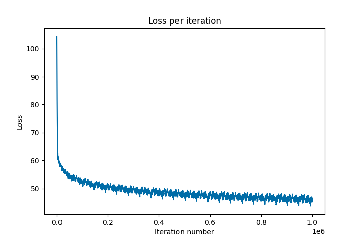
To achieve a more concrete understanding of model performance over time, the loss is plotted over a million training iterations for the initial single-layer RNN. After consistent decrease in loss at the beginning, the seemed to plateau in terms of loss around a value of 40. The loss would still gradually decrease, but at a very slow rate and very inconsistently (moving up and down). This may indicate the weakness of our basic RNN architecture; our model may simply not be complex enough to fully capture the patterns in the data, or be susceptible to problems during training like the vanishing and exploding gradient problems (discussed in Section).

Discussion

Given the simplify of our implementation and the relatively small size of data and lack of compute, the RNN performs very well. Not only does it spell English words (or at least produce English-like output), but it is able to capture Shakespearean style and play structure with character names. However, there are some significant limitations that lead to room for improvement.

Limitations

RNNs are plagued by vanishing and exploding gradients slope of the loss function along the error curve, which may provide an explanation as to why our models could not progress to loss values below 40.

When the gradient is too small (vanishing), updates to the weight parameters until they become insignificant, which means that the model learns very slowly or not at all. Exploding gradients occur when the gradient is too large, creating an unstable model (NaN results).

These problems especially bad for the recursive structure of RNNs, as the same weights are applied recursively at each time step of the input sequence. This means that during backpropagation, the gradients of these weights are also applied recursively through time. Because the same weights are used at each time step, any small gradients become exponentially smaller as they are propagated through each time step (vanishing), and conversely, any large gradients become exponentially larger (exploding).

RNN-type networks with specialized architectures, such as Long Short-Term Memory (LSTM) units and Gated Recurrent Units (GRU) mitigate the vanishing and exploding gradient problems. This is done by adding mechanisms to allow the information to bypass the traditional path through the RNN. This means that the gradient has a shortcut where it can flow without being multiplied by the weight matrix at each time step, thus reducing the risk of vanishing or exploding. These architectures are also better at capturing long-term dependencies by using a “memory cell” that can maintain information in memory for long periods of time.

Conclusion

This project demonstrated the power of basic multivariable calculus concepts in terms of complex and relevant applications, namely language modeling. A deep understanding of neural networks is established from first principles, then expanded to multilayer networks and eventually recurrent networks. Based on this understanding, implementation and experimentation were conducted for the interesting problem of Shakespeare generation. Overall, this paper provided an opportunity to gain a deeper understanding of machine learning and to build a small but powerful application.

References

Appendix A: RNN Code

The full code for the RNN and 3-layer RNN can be found on Github. A GRU implementation is also included, although no GRU experiments were discussed in the paper (out of scope).

Model Outputs

KING.
Are you chis lose! Meat and the our that vistrers? Let not for where, dame my forsta 

----
iter 997100, loss: 44.43487950312566
----
  and shall of my heakse herrage, How shaid I thoughty sween dofl ampaut
    To kasw, of the fuld on alinion; the combay
    If o
    Te to-near hare the comery, not mach save you lagd thtures beace re 

DAMITBURO:
Cartser.

PRONICALIO:
Me,ser lonk efes me, sighes,
Se; doo thung
sir, she Inow I save,
Lord my you vy chewell sut
xay; and msoy ipe uither, I feaver! 

GLAMUSE:
As thou peasant kister,
he revere his this rrous,
To gentle,,
And vor gud!

DUDN VINCE:
All that now conly wath are bedy, our greacd afparfer po,
And vorn of d

MERCELIZIO:
As,
To sir goleadies thouby kon?

LAMANIS:
O'l lid, your comes tell, jetite whouf oul;
Uraty sut, to be not me trance thesinem
The jobreined yearsick.

----
iter 421000, loss: 44.14635583930259
----
 
House with a doy, new ade
bid but condesiegh as as Soor her againss clavk;
Arature make keart keel that sims all tome, where;
So had it prait, are is your make with the not