UDL Chapter 6 Problems

Problem 6.1

Show that the derivates of the least squares loss function in equation 6.5 are given by the equations in 6.7.

Each loss component:

$${\ell }_i=({\varphi }_0+{\varphi }_1{x}_i-y_i{)}^2$$

Derivatives:

$$\frac{\partial {\ell }_i}{\partial {\varphi }_0}=2({\varphi }_0+{\varphi }_1{x}_i-y_i)$$ $$\frac{\partial {\ell }_i}{\partial {\varphi }_1}=2({\varphi }_0+{\varphi }_1{x}_i-y_i)(x_i)$$

Problem 6.2

A surface is guaranteed to be convex if the eigenvalues of the Hessian $\mathbf{H}[\varphi ]$ are positive everywhere. In this case, the surface has a unique minimum, and optimization is easy. Find an algebraic expression for the Hessian matrix,

$$\mathbf{H}[\varphi ]=\left[\begin{array}{cc}\frac{{\partial }^{2}L}{\partial {\varphi }_0^2}& \frac{{\partial }^{2}L}{\partial {\varphi }_0\partial {\varphi }_1}\\ \frac{{\partial }^{2}L}{\partial {\varphi }_1\partial {\varphi }_0}& \frac{{\partial }^{2}L}{\partial {\varphi }_1^2}\end{array}\right]$$

for the linear regression model. Prove that this function is convex by showing that the eigenvalues are always positive. This can be done by showing that both the trace and determinant of the matrix are positive.

We have:

$${\ell }_i=({\varphi }_0+{\varphi }_1{x}_i-y_i{)}^2$$

Top left $(H_{1,1})$:

$$\begin{array}{rl}\frac{\partial {\ell }_i}{\partial {\varphi }_0}& =2({\varphi }_0+{\varphi }_1{x}_i-y_i)\\ \frac{{\partial }^2{\ell }_i}{\partial {\varphi }_0^2}& =2\end{array}$$

Bottom left ($H_{2,1}$):

$$\begin{array}{r}\frac{{\partial }^2{\ell }_i}{\partial {\varphi }_1{\varphi }_0}=2x_i\end{array}$$

Top right ($H_{1,2}$):

$$\begin{array}{rl}\frac{\partial {\ell }_i}{\partial {\varphi }_1}& =2x_i({\varphi }_0+{\varphi }_1{x}_i-y_i)\\ \frac{{\partial }^2{\ell }_i}{\partial {\varphi }_0{\varphi }_1}& =2x_i\end{array}$$

Bottom right ($H_{2,2}$):

$$\frac{{\partial }^2{\ell }_i}{\partial {\varphi }_1^2}=2x_i^2$$

So the result for a single point is:

$$\left[\begin{array}{cc}2& 2x_i\\ 2x_i& 2x_i^2\end{array}\right]$$

And the Hessian of the total loss is:

$$H[\varphi ]=\sum _{i=1}^I\left[\begin{array}{cc}2& 2x_i\\ 2x_i& 2x_i^2\end{array}\right]=\left[\begin{array}{cc}2I& 2\sum x_i\\ 2\sum x_i& 2\sum x_i^2\end{array}\right]$$

The trace is positive:

$$\text{tr}(H)=H_{1,1}+H_{2,2}=2I+2\sum x_i^2>0$$

The determinant is:

$$\det (H)=ad-bc=(2I)\left(2\sum x_i^2\right)-{\left(2\sum x_i\right)}^2=4I\sum x_i^2-4{\left(\sum x_i\right)}^2>0$$

Thus, the surface is convex.

Problem 6.3

Compute the derivatives of the least squares loss $L[\varphi ]$ with respect to the parameters ${\varphi }_0$ and ${\varphi }_1$ for the Gabor model.

$$\begin{array}{rl}L[\varphi ]& =\sum _{i=1}^I(f[x_i,\varphi ]-y_i{)}^2\\ & ={\left(\sin [{\varphi }_0+0.06\cdot {\varphi }_{1}x]\cdot \exp \left(-\frac{({\varphi }_0+0.06\cdot {\varphi }_1{x}_i{)}^2}{32.0}\right)-y_i\right)}^2\end{array}$$

Let:

$$\begin{array}{rl}{g}_i& ={\varphi }_0+0.06{\varphi }_1{x}_i\\ f_i& =\sin (g_i)\cdot \exp \left(-\frac{g_i^2}{32}\right)\end{array}$$

Then, we have

$$L[\varphi ]=\sum r_i^2$$

where $r_i=f_i-y_i$.

First, we can find:

$$\begin{array}{rl}\frac{\partial f_i}{\partial g_i}& =\cos (g_i)\exp \left(-\frac{g_i^2}{32}\right)+\sin (g_i)\exp \left(-\frac{g_i^2}{32}\right)\left(-\frac{2g_i}{32}\right)\\ & =\exp \left(-\frac{g_i^2}{32}\right)\left[\cos (g_i)+\sin (g_i)\left(-\frac{g_i}{16}\right)\right]\end{array}$$

using the product rule and chain rule.

So:

$$\begin{array}{r}\frac{\partial f_i}{\partial {\varphi }_0}=\frac{\partial f_i}{\partial g_i}\frac{\partial g_i}{\partial {\varphi }_0}=\exp \left(-\frac{g_i^2}{32}\right)\left[\cos (g_i)+\sin (g_i)\left(-\frac{g_i}{16}\right)\right](1)\end{array}$$

and

$$\frac{\partial f_i}{\partial {\varphi }_1}=\frac{\partial f_i}{\partial g_i}\frac{\partial g_i}{\partial {\varphi }_1}=\exp \left(-\frac{g_i^2}{32}\right)\left[\cos (g_i)+\sin (g_i)\left(-\frac{g_i}{16}\right)\right](0.06x_i)$$

Because $L[\varphi ]=\sum r_i^2$, for each of the parameters, we have

$$\frac{\partial L}{\partial {\varphi }_k}=2\sum r_i\frac{\partial f_i}{\partial {\varphi }_k}$$

So:

$$\frac{\partial L}{\partial {\varphi }_0}=2\sum (f_i-y_i)\exp \left(-\frac{g_i^2}{32}\right)\left[\cos (g_i)+\sin (g_i)\left(-\frac{g_i}{16}\right)\right]$$

and

$$\frac{\partial L}{\partial {\varphi }_1}=2\sum (f_i-y_i)\exp \left(-\frac{g_i^2}{32}\right)\left[\cos (g_i)+\sin (g_i)\left(-\frac{g_i}{16}\right)\right](0.06x_i)$$

Problem 6.4

The logistic regression model uses a linear function to assign an input $\mathbf{x}$ to one of two classes $y\in \{0,1\}$. For a 1D input and a 1D output, it has two parameters, ${\varphi }_0$ and ${\varphi }_1$, and is defined

$$Pr(y=1|x)=\text{sig}[{\varphi }_0+{\varphi }_{1}x]$$

where $\text{sig}[\bullet ]$ is the logistic sigmoid function.

• (i) Plot $y$ against $x$ for this model for different values of ${\varphi }_0$ and ${\varphi }_1$ and explain the qualitative meaning of each parameters.
• (ii) What is a suitable loss function for this model?
• (iii) Compute the derivatives of this loss function with respect to the parameters.
• (iv) Generate ten data points from a normal distribution with mean $-1$ and standard deviation $1$ and assign them to label $y=0$. Generate another ten data points from a normal distribution with mean $1$ and standard deviation $1$ and assign these the label $y=1$. Plot the loss as a heatmap in terms of the two parameters ${\varphi }_0$ and ${\varphi }_1$. (v) Is this loss function convex? How could you prove this?

(i) ${\varphi }_0$ controls the location of the centerpoint of the sigmoid function ($y=0.5$), ${\varphi }_1$ controls the slope of the transition.

(ii) Binary cross-entropy loss:

$$L[\varphi ]=\sum _{i=1}^I-(1-y_i)\log [1-\text{sig}[{\varphi }_0+{\varphi }_{1}x]]-y_i\log [\text{sig}[{\varphi }_0+{\varphi }_{1}x]]$$

(iii) Derivatives of the sigmoid function are:

$$\frac{\partial \text{sig}[z]}{\partial z}=\frac{\exp [-z]}{(1+\exp [-z]{)}^2}$$

It follows that the derivatives of the loss function are

$$\begin{array}{rl}\frac{\partial L}{\partial {\varphi }_0}& =\frac{\partial L}{\partial (\text{sig}[{\varphi }_0+{\varphi }_1{x}_i])}\frac{\partial (\text{sig}[{\varphi }_0+{\varphi }_1{x}_i])}{\partial {\varphi }_0+{\varphi }_1{x}_i}\frac{\partial ({\varphi }_0+{\varphi }_1{x}_i)}{\partial {\varphi }_0}\\ & =\sum _{i=1}^I\left(\frac{1-y_i}{1-\text{sig}[{\varphi }_0+{\varphi }_1{x}_i]}-\frac{y_i}{\text{sig}[{\varphi }_0+{\varphi }_{1}x]}\right)\frac{\exp [-{\varphi }_0-{\varphi }_1{x}_i]}{(1+\exp [-{\varphi }_0-{\varphi }_1{x}_i]{)}^2}\end{array}$$

and

$$\begin{array}{rl}\frac{\partial L}{\partial {\varphi }_0}& =\frac{\partial L}{\partial (\text{sig}[{\varphi }_0+{\varphi }_1{x}_i])}\frac{\partial (\text{sig}[{\varphi }_0+{\varphi }_1{x}_i])}{\partial {\varphi }_0+{\varphi }_1{x}_i}\frac{\partial ({\varphi }_0+{\varphi }_1{x}_i)}{\partial {\varphi }_1}\\ & =\sum _{i=1}^I\left(\frac{1-y_i}{1-\text{sig}[{\varphi }_0+{\varphi }_1{x}_i]}-\frac{y_i}{\text{sig}[{\varphi }_0+{\varphi }_{1}x]}\right)\frac{\exp [-{\varphi }_0-{\varphi }_1{x}_i]}{(1+\exp [-{\varphi }_0-{\varphi }_1{x}_i]{)}^2}\cdot x_i\end{array}$$

(iv)

import numpy as np
import matplotlib.pyplot as plt
 
np.random.seed(42)
 
# Generate data
x0 = np.random.normal(-1.0, 1.0, 10)
y0 = np.zeros(10)
 
x1 = np.random.normal(1.0, 1.0, 10)
y1 = np.ones(10)
 
x = np.concatenate([x0, x1])
y = np.concatenate([y0, y1])
 
# Sigmoid and loss
def sigmoid(z):
    return 1 / (1 + np.exp(-z))
 
def loss(phi0, phi1):
    z = phi0 + phi1 * x
    p = sigmoid(z)
    eps = 1e-12
    p = np.clip(p, eps, 1 - eps) # Keep p from exact 0 or 1 to prevent overflow
    return -np.sum((1 - y) * np.log(1 - p) + y * np.log(p))
 
# Grid
phi0_vals = np.linspace(-4, 4, 200)
phi1_vals = np.linspace(-4, 4, 200)
loss_grid = np.zeros((len(phi1_vals), len(phi0_vals)))
 
for i, phi1 in enumerate(phi1_vals):
    for j, phi0 in enumerate(phi0_vals):
        loss_grid[i, j] = loss(phi0, phi1)
 
# Plot
plt.figure(figsize=(7, 6))
plt.imshow(
    loss_grid,
    extent=[phi0_vals.min(), phi0_vals.max(), phi1_vals.min(), phi1_vals.max()],
    origin="lower",
    aspect="auto",
)
 
# Add level curves (contours)
min_loss = np.min(loss_grid)
max_loss = np.max(loss_grid)
contour_levels = np.linspace(min_loss, max_loss, 15)
plt.contour(
    phi0_vals, 
    phi1_vals, 
    loss_grid, 
    levels=contour_levels,
    colors='white',
    alpha=0.7,
    linewidths=0.5
)
 
plt.colorbar(label="Loss")
plt.xlabel(r"$\phi_0$")
plt.ylabel(r"$\phi_1$")
plt.title("Binary Cross‑Entropy Loss Surface")
plt.show()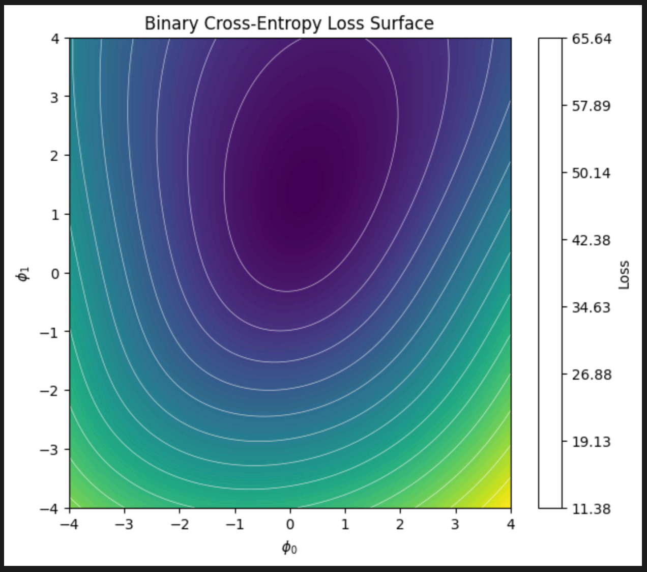

(v) The loss function seems to be convex based on the plot above. We can prove it by examining the Hessian matrix like we did in question 6.2.

Problem 6.5

Compute the derivatives of the least squares loss with respect to the ten parameters of the simple neural network model:

$$f[x,\varphi ]={\varphi }_0+{\varphi }_{1}a[{\theta }_{10}+{\theta }_{11}x]+{\varphi }_2[{\theta }_{20}+{\theta }_{21}x]+{\varphi }_{3}a[{\theta }_{30}+{\theta }_{31}x]$$

Think carefully about what the derivative of the ReLU function $a[\bullet ]$ will be.

The derivative of the least squares loss function $f[x,\varphi ]$ is given by:

$$\frac{\partial L}{\partial {\varphi }_j}=-2\sum _i(y-f[x_i,\varphi ])\frac{\partial f[x_i,\varphi ]}{\partial {\varphi }_j}$$

The derivative of ReLU is:

$$\{\begin{array}{ll}0& \text{if }z<0\\ 1& \text{if }z>0\end{array}$$

We can write this as $\mathbb{I}[z>0]$.

Then, the derivatives are:

$$\begin{array}{rl}\frac{\partial f[x_i,\varphi ]}{\partial {\varphi }_0}& =1\\ \frac{\partial f[x_i,\varphi ]}{\partial {\varphi }_1}& =a[{\theta }_{10}+{\theta }_{11}{x}_i]\\ \frac{\partial f[x_i,\varphi ]}{\partial {\varphi }_2}& =a[{\theta }_{20}+{\theta }_{21}{x}_i]\\ \frac{\partial f[x_i,\varphi ]}{\partial {\varphi }_3}& =a[{\theta }_{30}+{\theta }_{31}{x}_i]\end{array}$$

and:

$$\begin{array}{rl}\frac{\partial f[x_i,\varphi ]}{\partial {\theta }_{10}}& ={\varphi }_1\cdot \mathbb{I}[{\theta }_{10}+{\theta }_{11}{x}_i>0]\\ \frac{\partial f[x_i,\varphi ]}{\partial {\theta }_{11}}& ={\varphi }_1\cdot x_i\cdot \mathbb{I}[{\theta }_{10}+{\theta }_{11}{x}_i>0]\\ \frac{\partial f[x_i,\varphi ]}{\partial {\theta }_{20}}& ={\varphi }_2\cdot \mathbb{I}[{\theta }_{20}+{\theta }_{21}{x}_i>0]\\ \frac{\partial f[x_i,\varphi ]}{\partial {\theta }_{21}}& ={\varphi }_2\cdot x_i\cdot \mathbb{I}[{\theta }_{20}+{\theta }_{21}{x}_i>0]\\ \frac{\partial f[x_i,\varphi ]}{\partial {\theta }_{30}}& ={\varphi }_3\cdot \mathbb{I}[{\theta }_{30}+{\theta }_{31}{x}_i>0]\\ \frac{\partial f[x_i,\varphi ]}{\partial {\theta }_{31}}& ={\varphi }_3\cdot x_i\cdot \mathbb{I}[{\theta }_{30}+{\theta }_{31}{x}_i>0]\end{array}$$

Problem 6.6

Which of the functions in figure 6.11 is convex? Justify your answer. Character each of the points 1-7 as (i) a local minimum, (ii) a global minimum, or (iii) neither.

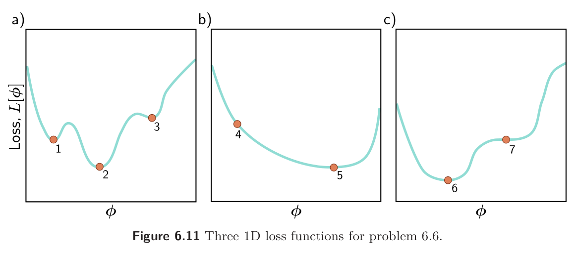
B is the only convex function; all chords lie below above the function. A is non-convex (a chord from 1 → 2 or 2 → 3 would be below the curve), C is non-convex (a chord from 6 → 7 would intersect/be below the curve).

Points:

1. Local minimum
2. Global minimum
3. Local minimum
4. Neither
5. Global minimum
6. Global minimum
7. Neither (saddle point)

Problem 6.7

The gradient descent trajectory for path 1 in figure 6.5a oscillates back and forth inefficiently as it moves down the valley toward the minimum. It’s also notable that it turns at right angles to the previous direction at each step. Provide a qualitative explanation for these phenomena. Propose a solution that might help prevent this behavior.

The trajectory must turn at right angles. If the current direction still had any component pointing downhill (i.e. decreasing the function), we should logically keep going in that direction. However, we’re in a “curved valley” and just overshot the center, so continuing in the same direction would now move you uphill on the other side, so the gradient reverses direction sharply.

Solutions include Newton’s method (use second derivative to understand curvature of the loss landscape) or momentum.

Problem 6.8

Can (non-stochastic) gradient descent with a fixed learning rate escape local minima?

No - in a local minima the gradient will be zero or near zero so the non-stochastic gradient descent will just be stuck there as it has no reason to move.

Problem 6.9

We run the stochastic gradient descent algorithm for 1000 iterations on a dataset of size 100 with a batch size of 20. For how many epochs did we train the model?

Batch size of 20, total size 100 means that 1 epoch is 100/20 = 5 iterations. 1000/5 = 200 epochs.

Problem 6.10

Show that the momentum term ${\mathbf{m}}_t$ (equation 6.11) is an infinite weighted sum of the gradients at the previous iterations and derive an expression for the coefficients (weights) of that sum.

Recall that the momentum update is given by

$$\begin{array}{rl}{\mathbf{m}}_{t+1}& =\beta \cdot {\mathbf{m}}_t+(1-\beta )\sum _{i\in {\mathcal{B}}_t}\frac{\partial {\ell }_i[{\varphi }_t]}{\partial \varphi }\\ & =\beta \cdot {\mathbf{m}}_t+(1-\beta )\cdot {\mathbf{g}}_t\end{array}$$

We want to unroll this sequence.

$$\begin{array}{rl}{\mathbf{m}}_{t+1}& =\beta \cdot (\beta \cdot {\mathbf{m}}_{t-1}+(1-\beta ){\mathbf{g}}_{t-1})+(1-\beta )\cdot {\mathbf{g}}_t\\ & ={\beta }^2\cdot {\mathbf{m}}_{t-1}+\beta (1-\beta )\cdot {\mathbf{g}}_{t-1}+(1-\beta )\cdot {\mathbf{g}}_t\\ & ={\beta }^3\cdot {\mathbf{m}}_{t-2}+{\beta }^2(1-\beta )\cdot {\mathbf{g}}_{t-2}+\beta (1-\beta )\cdot {\mathbf{g}}_{t-1}+(1-\beta ){\mathbf{g}}_t\\ & ={\beta }^{t+1}{\mathbf{m}}_0+\sum _{k=0}^t(1-\beta ){\beta }^k\cdot {\mathbf{g}}_{t-k}\end{array}$$

Thus, as $t\to \infty$, this sum approaches an infinite sum of the form:

$$m_{t+1}=\sum _{k=0}^{\infty }{w}_k{g}_{t-k}$$

where $w_k=(1-\beta ){\beta }^k$.

Problem 6.11

What dimensions will the Hessian have if the model has one million parameters?

The Hessian will be $1\text{ million }\times \text{1 million}$:

$$H\in {\mathbb{R}}^{10^6\times 10^6}$$