Conditional Probabilistic Perspective of Learning

Consider a model $f[x,\varphi ]$ with parameters $\varphi$ that computes an output from $x$. Instead of thinking about the model directly computing a prediction $y$, we can shift perspective and consider the model as computing a conditional probability distribution $Pr(y|x)$, over possible outputs $y$ given $x$.

The loss encourages each training output $y_i$ to have a high probability under the distribution $Pr(y_i|x_i)$, computed from the corresponding $x_i$.

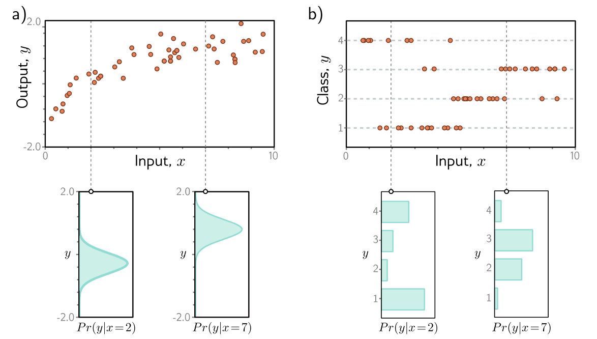
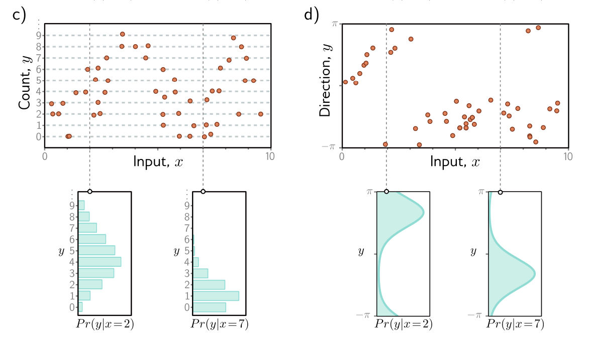
Conditional probability model examples

!>Maximum Likelihood for Loss Functions-20250609235217601.png

• a) Regression task, where the goal is to predict a real-valued output $y$ from the input $x$ based on training data $\{x_i,y_i\}$ (orange points). For each input value x, the model predicts a distribution $Pr(y|x)$ over the output $y\in R$. The loss function aims to maximize the probability of the observed training outputs $y_i$ under the distribution predicted from the corresponding inputs $x_i$.
• b) To predict discrete classes $y\in \{1,2,3,4\}$ in a classification task, we use a discrete probability distribution, so the model predicts a different histogram over the four possible values of $y_i$ for each value of $x_i$.

• c) To predict counts $y\in \{0,1,2,\dots \}$ we use distributions defined over positive integers
• d) To predict directions $y\in (-\pi ,\pi ]$, we use distributions defined over circular domains

Computing a distribution over outputs

How exactly can a model $f(x,\varphi )$ be adapted to compute a probability distribution?

First, we choose a parametric distribution $Pr(y|\theta )$ defined on the output domain $y$. Then, we use the network to compute one or more of the parameters $\theta$ of this distribution.

For example, suppose the prediction domain is the set of real numbers, so $y\in \mathbb{R}$. Here, we might choose the univariate normal distribution, which is defined on $\mathbb{R}$. This distribution is defined by the mean $\mu$ and variance ${\sigma }^2$, so $\theta =\{\mu ,{\sigma }^2\}$. The model might predict the mean $\mu$, and the variance ${\sigma }^2$ could be treated as an unknown constant.

Inference

We use log-likelihood as a loss function to find the best parameters. At inference time, the network no longer predicts the outputs $y$ but instead determines a probability distribution over $y$. However, we often want to use a point estimate rather than a distribution.

To do this, we return the maximum of the distribution

$$\hat{y}=\underset{y}{\mathrm{argmax}}[Pr(y|f(x,\hat{\varphi }))]$$

It’s usually possible to find an expression for this in terms of the distribution parameters $\theta$ predicted by the model. For example, in the univariate normal distribution, the maximum occurs at the mean $\mu$.

Multiple Outputs

Often, we wish to make more than one prediction with the same model, so the target output $\mathbf{y}$ is a vector. For example, we might want to predict a molecule’s melting and boiling point (multivariate regression), or the obstacle class at every point in an image (multivariate classification). While it’s possible to define multivariate probability distributions and use a neural network to model their parameters as a function of the input, it’s more usual to treat each prediction as independent.

Independence implies that we treat the probability $Pr(\mathbf{y}|\mathbf{f}[\mathbf{x},\varphi ])$ as a product of variate terms for each element $y_d\in \mathbf{y}$:

$$Pr(\mathbf{y}|\mathbf{f}[\mathbf{x},\varphi ])=\prod _{d}Pr(y_d|{\mathbf{f}}_d[\mathbf{x},\varphi ])$$

where ${\mathbf{f}}_d[\mathbf{x},\varphi ]$ is the $d$-th set of network outputs, which describe the parameters of the distribution over $y_d$. For example:

• To predict multiple continuous variables $y_d\in \mathbb{R}$, we use a normal distribution for each $y_d$, and the network outputs $f_d[\mathbf{x},\varphi ]$ predict the means of these distributions.
• To predict multiple discrete variables $y_d\in \{1,2,\dots ,K\}$, we use a categorical distribution for each $y_d$. Here, each set of network outputs ${\mathbf{f}}_d[\mathbf{x},\varphi ]$ predicts the $K$ values that contribute to the categorical distribution for $y_d$.

When we minimize the negative log-likelihood, this product becomes a sum of terms:

$$L[\varphi ]=-\sum _{i=1}^I\log [Pr({\mathbf{y}}_i|\mathbf{f}[{\mathbf{x}}_i,\varphi ])]=-\sum _{i=1}^I\sum _d\log [Pr(y_{id}|{\mathbf{f}}_d[{\mathbf{x}}_i,\varphi ])]$$

where $y_{id}$ is the $d$-th output from the $i$-th training example.

To make two or more prediction types simultaneously, we similarly assume the errors in each are independent.

• Example: To predict wind direction and strength, we might choose the von Mises distribution (defined on circular domains) for the direction, and the exponential distribution (defined on positive real numbers) for the strength.

The independence assumption implies that the joint likelihood of the two predictions if the product of individual likelihoods. These terms will become additive when we compute the negative log-likelihood.