MATLAB Worksheet 2

Question 1

1a.

We can find $a$ and $b$ by comparing the coordinate values of $P_0$ and $P_f$ with the components of $\vec{r}(t)$. This is simple since the $\vec{i}$ component of $\vec{r}(t)$ is just $t$, such that:

$$\vec{i}:a=P_{0x}=-\frac{1}{2}$$

We can check this against the $\vec{j}$ and $\vec{k}$ components to verify if they are correct:

$$\begin{array}{rl}& \vec{j}:\sqrt{3}a=\sqrt{3}\left(-\frac{1}{2}\right)=-\frac{\sqrt{3}}{2}\\ & \vec{k}:1.5a^2-0.25a=1.5{\left(-\frac{1}{2}\right)}^2-0.25\left(-\frac{1}{2}\right)=\frac{1}{2}\end{array}$$

Similarly for $b$ and $P_f$:

$$\begin{array}{rl}& \vec{i}:b=P_{fx}=\frac{3}{2}\\ & \vec{j}:\sqrt{3}a=\sqrt{3}\left(\frac{3}{2}\right)=\frac{3\sqrt{3}}{2}\\ & \vec{k}:1.5a^2-0.25a=1.5{\left(\frac{3}{2}\right)}^2-0.25\left(\frac{3}{2}\right)=3\end{array}$$

Thus, we have confirmed:

$$\boxed{\begin{array}{rl}a& =-\frac{1}{2}\\ b& =\frac{3}{2}\end{array}}$$

1b.

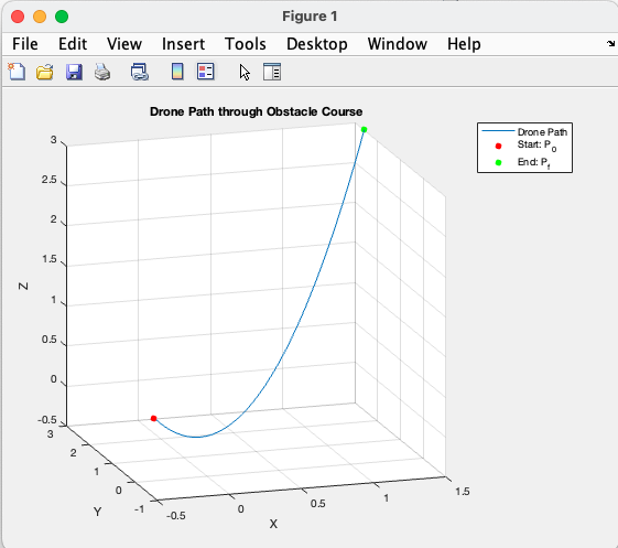
t = linspace(-1/2, 3/2, 1000);
 
x = t;
y = sqrt(3)*t;
z = 1.5*t.^2 - 0.25*t;
 
figure;
 
plot3(x, y, z, 'DisplayName', 'Drone Path')
hold on;
 
scatter3(-1/2, -sqrt(3)/2, 1/2, 'o', 'r', 'filled', 'DisplayName', 'Start: P_0')
scatter3(3/2, 3*sqrt(3)/2, 3, 'o', 'g', 'filled', 'DisplayName', 'End: P_f')
 
xlabel('X')
ylabel('Y')
zlabel('Z')
title('Drone Path through Obstacle Course')
 
grid on;
legend;
hold off;

Question 2

2a.

syms t
 
x = t;
y = sqrt(3)*t;
z = 1.5*t^2 - 0.25*t;
 
dx_dt = diff(x, t);
dy_dt = diff(y, t);
dz_dt = diff(z, t);
 
integrand = sqrt(dx_dt^2 + dy_dt^2 + dz_dt^2);
 
arc_length_symbolic = int(integrand, t, -1/2, 3/2);
 
arc_length_numeric = double(arc_length_symbolic);
 
disp(['Arc Length: ', num2str(arc_length_numeric), ' km'])
Arc Length: 5.6278 km

2b.

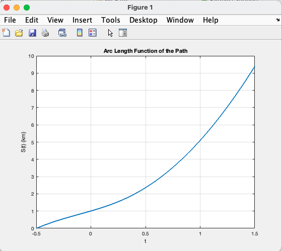
syms t u
 
x = t;
y = sqrt(3)*t;
z = 1.5*t^2 - 0.25*t;
 
dx_dt = diff(x, t);
dy_dt = diff(y, t);
dz_dt = diff(z, t);
 
speed = sqrt(dx_dt^2 + dy_dt^2 + dz_dt^2);
 
S = int(speed, u, -1/2, t);
S = matlabFunction(S); % Convert symbolic expression to function handle
 
t_vals = linspace(-1/2, 3/2, 1000);
S_vals = arrayfun(S, t_vals);
 
figure;
plot(t_vals, S_vals, 'LineWidth', 2);
xlabel('t');
ylabel('S(t) (km)');
title('Arc Length Function of the Path');
grid on;

2c.

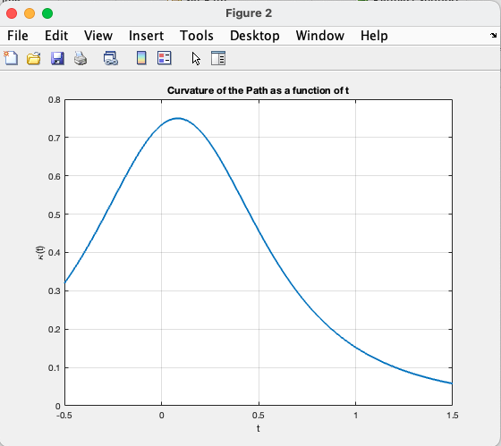
syms t
 
x = t;
y = sqrt(3)*t;
z = 1.5*t^2 - 0.25*t;
 
dx_dt = diff(x, t);
dy_dt = diff(y, t);
dz_dt = diff(z, t);
 
d2x_dt2 = diff(dx_dt, t);
d2y_dt2 = diff(dy_dt, t);
d2z_dt2 = diff(dz_dt, t);
 
magnitude_cross_product = sqrt((dy_dt*d2z_dt2 - dz_dt*d2y_dt2)^2 + ...
                              (dz_dt*d2x_dt2 - dx_dt*d2z_dt2)^2 + ...
                              (dx_dt*d2y_dt2 - dy_dt*d2x_dt2)^2);
 
magnitude_r_prime_cubed = (sqrt(dx_dt^2 + dy_dt^2 + dz_dt^2))^3;
 
kappa = magnitude_cross_product / magnitude_r_prime_cubed;
kappa = simplify(kappa); % Simplify the curvature function
 
kappa_func = matlabFunction(kappa);
 
t_vals = linspace(-1/2, 3/2, 1000);
kappa_vals = arrayfun(kappa_func, t_vals);
 
figure;
plot(t_vals, kappa_vals, 'LineWidth', 2);
xlabel('t');
ylabel('\kappa(t)');
title('Curvature of the Path as a function of t');
grid on;

2d.

A suitable path would have low and smooth curvature in order to avoid sudden changes in acceleration. We can quantitatively analyze the acceleration by finding the magnitude of the second derivative of $\vec{r}(t)$. First we can parametrize $\vec{r}(t)$ so that we have:

$$\begin{array}{rl}x(t)& =t\\ y(t)& =\sqrt{3}t\\ z(t)& =1.5t^2-0.25t\end{array}$$

Taking the second derivatives we have:

$$\begin{array}{rl}{x}^{\prime \prime }(t)& =0\\ y^{\prime \prime }(t)& =0\\ z^{\prime \prime }(t)& =3\end{array}$$

Thus, the magnitude the acceleration vector ${\vec{r}}^{\prime \prime }(t)=⟨0,0,3⟩$ is just constant at $3\text{ m/s}$. This is a suitable drone path because there are no sudden changes in acceleration. However, it should be considered whether the acceleration of $3\text{ m/s}$ is too high, which can be a concern due to increased power consumption, potential instability, and increased wear and tear on components.

Question 3

3a.

fun = @(p) cos(p(1)) + sin(p(2));
 
limits = [-10, 10];
 
results_table = table();
 
% Generate 10 random guesses
for i = 1:10
    x0 = limits(1) + (limits(2) - limits(1)).*rand();
    y0 = limits(1) + (limits(2) - limits(1)).*rand();
    
    [p_min, f_min] = fminsearch(fun, [x0, y0]);
    
    temp_table = table(x0, y0, p_min(1), p_min(2), f_min, 'VariableNames', {'x0', 'y0', 'xmin', 'ymin', 'f_xmin_ymin'});
    results_table = [results_table; temp_table];
end
disp(results_table);
 
      x0         y0        xmin       ymin      f_xmin_ymin
    _______    _______    _______    _______    ___________
 
     3.1148    -9.2858     3.1416     -7.854        -2     
     6.9826     8.6799     9.4248     10.996        -2     
     3.5747     5.1548     3.1416     4.7124        -2     
     4.8626    -2.1555     3.1416    -1.5708        -2     
     3.1096    -6.5763     3.1416     -7.854        -2     
     4.1209    -9.3633     3.1416    -7.8539        -2     
    -4.4615    -9.0766    -3.1416     -7.854        -2     
    -8.0574     6.4692    -9.4248     4.7124        -2     
     3.8966     -3.658     3.1416    -1.5708        -2     
     9.0044    -9.3111     9.4247     -7.854        -2  

3b.

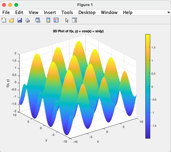
[x, y] = meshgrid(linspace(-10, 10, 400)); 
z = cos(x) + sin(y); 
 
surf(x, y, z, 'EdgeColor', 'none'); 
xlabel('x'); 
ylabel('y'); 
 
zlabel('f(x, y)');
title('3D Plot of f(x, y) = cos(x) + sin(y)'); 
colorbar;

When comparing the plot and the results from part (a), it seems that fminsearch converges to local minima of $-2$ in various places in the domain. The function $f(x,y)=\cos (x)+\sin (y)$ has multiple local minima, which makes sense as both sine and cosine functions are periodic but they have minima at different points. As far as I know, there is no way we can address the problem with fminsearch for this particular function due to its periodic nature.