The case against deep learning
Deep learning works unreasonably well – it is surprising the deep networks are easy to train and also surprising that they generalize.
With sufficient hidden units, deep networks will classify almost any training set near-perfectly. Performance of a 2-layer FC network on 10000 MNIST-1D training examples is perfect once there are 43 hidden units per layer or ~4000 parameters. However, finding the global minimum of an arbitrary non-convex function is NP-hard, and this is also true for certain neural network loss functions. It’s remarkable that the fitting algorithm doesn’t get trapped in local minima or stuck near saddle points, and that it can efficiently recruit spare model capacity to fit unexplained training data wherever they lie.
This is not as surprising when there are a lot more parameters than training data, but it can still be true when this is not the case. GPT-3 had 175 billion parameters and was trained with 300 billion tokens; not that over-parameterized.
The ability of DNNs to fit neural networks efficiently is even more startling. It’s not obvious that typical datasets are sufficient to characterize the input/output mapping. The Curse of Dimensionality implies that the training dataset is tiny compared to the space of all possible inputs.
Also, DNNs describe very complicated functions. A fully connected network for MNIST-1D with two hidden layers of width 400 can create mappings with up to linear regions. That’s regions per training example, so very few of these regions contain data at any stage during training; regardless, those regions that do encounter data points constrain the remaining regions to behave reasonably.
Generalization gets better with more parameters (double descent). This is surprising, since more parameters means that the model can do almost anything between the training data, but is able to behave sensibly.
What might explain the unexpected performance of deep networks?
Data
It’s important to realize that we can’t learn any function. Consider a completely random mapping from every possible binary image to one of ten categories. Since there is no structure to the function, the only recourse is to memorize the assignments. However, it’s easy to train a model on MNIST, which contains 60,000 examples of images labeled with one of 10 categories. This might be because it is relatively simple to find global minima.
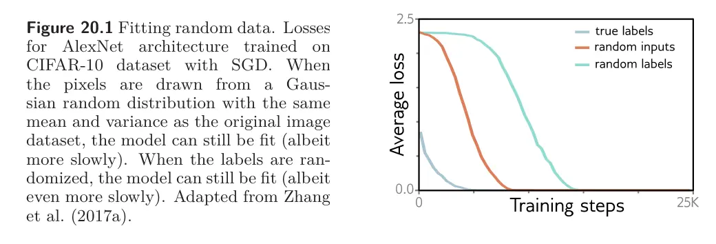
However, the properties of the dataset also aren’t critical. Consider AlexNet on CIFAR-10; when each image is replaced with Gaussian noise and the labels are randomly permuted, learning slowed down, but the network could still fit the finite dataset well.
Regularization
Another possible explanation for the ease with which models are trained is that some regularization methods like L2 Regularization make the loss surface flatter and more convex. However, it has been found that neither L2 regularization nor Dropoutis required to fit random data. This does not eliminate implicit regularization due to the finite step size of fitting algorithms; but this effect should increase with learning rate yet model-fitting does not get easier with larger learning rates.
Stochastic training algorithms
SGD potentially allows the optimization trajectory to move between “valleys” during training. However, it has been that several models can be fit to many datasets almost perfectly, which eliminates most of the randomness, but training still succeeds.
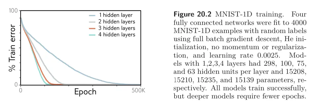
The figure below shows four fully connected models fitted to 4000 MNIST-1D examples with randomized labels using full-batch (non-stochastic) gradient descent. There was no explicit regularization, and the learning rate was set to a small constant value to minimize implicit regularization. Here, the true mapping from data to labels has no structure, the training is deterministic, and there is no regularization, yet the training error still decreases to zero. This suggests that these loss functions may genuinely have no local minima.
Overparameterization
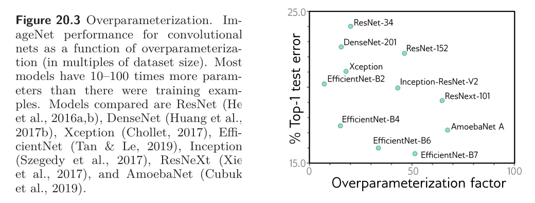
Overparameterization almost certainly is an important factor that contributes to ease of training. It implies that there is a large family of degenerate solutions, so there may always be a direction in which the parameters can be modified to decrease the loss. “The degeneracy of solutions changes the nature of the problem from finding a needle in a haystack to a haystack of needles.”
In practice, networks are frequently overparameterized by one or two orders of magnitude. However, data augmentation makes it difficult to make precise statements. Augmentation may increase the data by several orders of magnitude, but these are manipulations of existing examples rather than independent data points. Moreover, it has been shown that networks can sometimes fit the training data well when there are the same number of fewer parameters than data points. This is presumably due to redundancy in training examples from the same underlying function.
Several theoretical convergence results show that, under certain circumstances, SGD converges to a global minimum when the network is sufficiently overparameterized. For example, analysis has been done on:
- Randomly initialized SGD converges to a global minimum for shallow fully connected ReLU networks with a least squares loss with enough hidden units.
- Deep, residual and convolutional networks converge when the activation function is smooth and Lipschitz
- Convergence of gradient descent on deep, fully connected networks using hinge loss
If a neural network is sufficiently overparameterized so that it can memorize any dataset of a fixed size, then all the stationary points become global minima. Other results show that if the network is wide enough, local minima where the loss is higher than the global minimum are rare. It has also been proven that as a network becomes deeper, wider, or both, the loss at local minima becomes closer to that at the global minimum for squared loss functions.
These theoretical results are intriguing but usually make unrealistic assumptions about the network structure. Thus, overparameterization seems to be important, but theory cannot yet explain empirical fitting performance.
Activation functions
The activation function is also known to affect training difficulty. Networks where the activation only changes over a small part of the input range are harder to hit than ReLUs (which vary over half the input range) or Leaky ReLUs (which vary over the full range). For example, sigmoid and tanh nonlinearities have shallow gradients in their tails; where the activation function is near constant, the training gradient is near zero, so the mechanism to improve the model is extremely weak.
Initialization
Another potential explanation is that Xavier/He initialization sets the parameters to values that are easy to optimize. Of course, for deeper networks, such initialization is necessary to avoid exploding and vanishing gradients, so in a trivial sense, initialization is critical to training success.
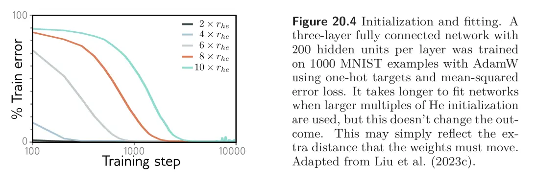
For shallower networks, the initial variance of the weights is less important. As the variance increases from that proposed by He, more iterations are required to fit the training data, but it usually does not ultimately impede fitting. Hence, initialization doesn’t shed much light on why fitting neural networks is easy, although exploding/vanishing gradients do reveal initializations that make training difficult with finite precision arithmetic.
Network depth
Neural networks are harder to fit when the depth becomes very large due to exploding gradients and shattered gradients. However, these are arguably practical numerical issues. There is no definitive evidence that the underlying loss function is fundamentally more or less convex as the network depth increases. There has been evidence (see figure below) that deeper networks train in fewer iterations. However, this might be because either (i) the gradients in deeper networks are steeper or (ii) He initialization just starts wider, shallower networks further away form the optimal parameters.
The network depth might also be relevant in terms of the Lottery Ticket Hypothesis.