Changing Growth Rates

Dividends tend to grow at different rates depending on where the company is in its life cycle, economy, availability of positive NPV projects, cash flow uncertainty, etc. Thus, it may be more realistic to use a differential (rather than zero or constant) dividend growth approach.

To do this, we estimate dividends as closely as possible in the foreseeable future, and assume constant growth rate thereafter:

$$P_0=\underset{\text{Precise valuation for short-term dividends}}{\underbrace{\frac{D_1}{1+r_E}+\frac{D_2}{(1+r_E{)}^2}+\cdots +\frac{D_N}{1+(r_E{)}^N}}}+\underset{\text{Growing perpetuity}}{\underbrace{\frac{D_N(1+g)}{r_E-g}\frac{1}{(1+r_E{)}^N}}}$$

So, we use a two-step in computing the stock price of non-constant growth rates

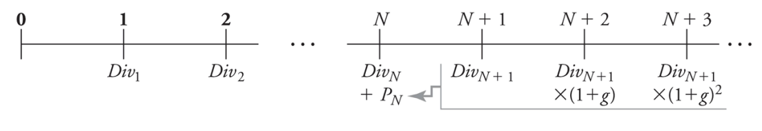
1. Compute terminal value by applying the constant growth model to calculate the future share price of the stock once the expected growth rate stabilizes:

$$P_N=\frac{Di{v}_{N+1}}{r_E-g}$$

2. Add the other non–constant dividends:

$$\begin{array}{rl}{P}_0& =\frac{Di{v}_1}{1+r_E}+\frac{Di{v}_2}{(1+r_E{)}^2}+\cdots +\frac{Di{v}_N}{(1+r_E{)}^N}+\frac{1}{(1+r_E{)}^N}{P}_N\\ & =\frac{Di{v}_1}{1+r_E}+\frac{Di{v}_2}{(1+r_E{)}^2}+\cdots +\frac{Di{v}_N}{(1+r_E{)}^N}+\frac{1}{(1+r_E{)}^N}\left(\frac{Di{v}_{N+1}}{r_E-g}\right)\end{array}$$

Example

Small Fry, Inc., has just invented a potato chip that looks and tastes like a french fry. Given the phenomenal market response to this product, Small Fry is reinvesting all of its earnings to expand its operations. Earnings were $2 per share this past year and are expected to grow at a rate of 20% per year until the end of year 4. At that point, other companies are likely to bring out competing products. Analysts project that at the end of year 4, Small Fry will cut its investment and begin paying 60% of its earnings as dividends. Its growth will also slow to a long-run rate of 4%. If Small Fry’s equity cost of capital is 8%, what is the value of a share today?

First, we use the projected earnings growth rate and payout rate to forecast its future earnings and dividends for year 1-4. Then, we find the constant growth dividends for year 5 and later:

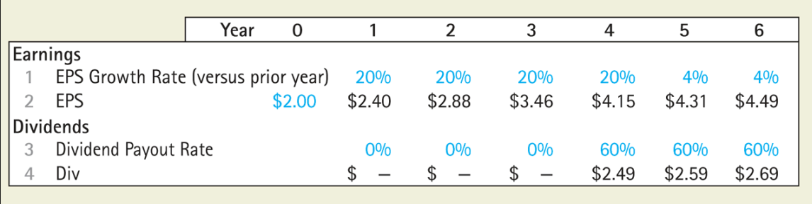
We can find dividends after year 4 with

$$D_5=D_4(1+4\%)=2.59$$

Now, we can use the terminal value of the stock at year 4 using constant growth dividends starting from year 5:

$$P_4=\frac{Di{v}_5}{r_E-g}=\frac{2.49(1+0.04)}{0.08-0.04}=64.74$$

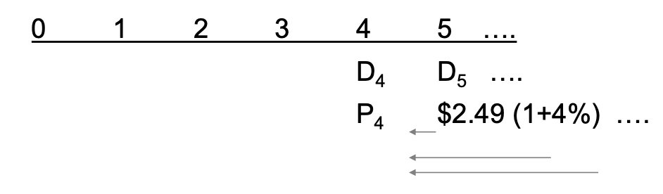
Then, we can compute the PV of other dividends and $P_4$:

$$P_0=\frac{Di{v}_1}{1+r_E}+\frac{Di{v}_2}{(1+r_E{)}^2}+\frac{Di{v}_3}{(1+r_E{)}^3}+\frac{Di{v}_4}{(1+r_E{)}^4}+\frac{P_4}{(1+r_E{)}^4}=49.42$$